Quasidynamic earthquake cycles on two faults
Contents
7. Quasidynamic earthquake cycles on two faults
7.1. Summary
Much like the last section, we simulate quasidynamic rupture evolution but this time on two faults, one of which is curved.
Most of the code here follows almost exactly from the previous section on strike-slip/antiplane earthquake cycles.
Realistic tectonic loading is a challenge when there is more than one fault.
The boundary integral approach used here is barely more complex with two faults than with one fault.
7.2. Loading a multi-fault system
In the single fault system from the last section, we were able to gloss over loading by using a slip deficit or backslip formulation. Because the physical system is invariant with respect to a rigid body displacement, any tectonic motion that has already been fully accomodated by fault slip can be ignored. Put differently, in a single fault system with a purely elastic rheology, the stresses from tectonic motion can be equivalently described by backwards slip on the fault.
There are a number of different options for loading a fault system:
backslip: as discussed, we simply apply a backwards slip rate to account for distant plate motion. Once the stresses from this backwards slip accumulate, the fault slips forward.
farfield displacement: apply a constant velocity boundary condition at a distance from the fault.
stress: Either on a lower boundary of the domain or on distant side boundaries, apply a constant traction/stress loading rate.
block model: this is a more advanced version of backslip loading where each fault-bounded subregion of the domain has its own block rotation/motion rate. These rates are assumed to be the long term slip rate. A corresponding kinematic slip deficit is applied to each fault.
Here, I do something a bit like the block model solution by just applying a backslip of 31 mm of loading per year (1 nm of loading per second) to both faults equally. This would model a real-world situation with a plate boundary that has 62 mm per year of strike-slip motion. Exactly 50% of that motion is accomodated by each of the two faults.
import sympy as sp
import numpy as np
import matplotlib.pyplot as plt
from tectosaur2 import (
    gauss_rule,
    integrate_term,
    panelize_symbolic_surface,
    concat_meshes,
)
from tectosaur2.laplace2d import double_layer, hypersingular
shear_modulus = 3.2e10
quad_rule = gauss_rule(5)
t = sp.var("t")
fault_bottom = 40000
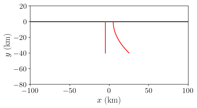
fault1 = panelize_symbolic_surface(
t, -5000 + t * 0, fault_bottom * (t + 1) * -0.5,
quad_rule,
n_panels=200
)
fault2_x = 5000 + (t * 10000 + 10000) + (t ** 2 * 5000 - 5000)
fault2 = panelize_symbolic_surface(
t, fault2_x, fault_bottom * (t + 1) * -0.5,
quad_rule,
n_panels=200
)
faults = concat_meshes((fault1, fault2))
surf_half_L = 100000
free = panelize_symbolic_surface(
t, -t * surf_half_L, 0 * t,
quad_rule,
n_panels=200
)
print(
    f"The free surface mesh has {free.n_panels} panels with a total of {free.n_pts} points."
)
print(
    f"The fault mesh has {faults.n_panels} panels with a total of {faults.n_pts} points."
)
The free surface mesh has 200 panels with a total of 1000 points.
The fault mesh has 400 panels with a total of 2000 points.
plt.plot(free.pts[:,0]/1000, free.pts[:,1]/1000, 'k-')
plt.plot(fault1.pts[:,0]/1000, fault1.pts[:,1]/1000, 'r-')
plt.plot(fault2.pts[:,0]/1000, fault2.pts[:,1]/1000, 'r-')
plt.xlabel(r'$x ~ \mathrm{(km)}$')
plt.ylabel(r'$y ~ \mathrm{(km)}$')
plt.axis('scaled')
plt.xlim([-100, 100])
plt.ylim([-80, 20])
plt.show()
singularities = np.array(
    [
        [-surf_half_L, 0],
        [surf_half_L, 0],
        [5000, 0],
        [-5000, 0]
    ]
)

(free_disp_to_free_disp, fault_slip_to_free_disp), report = integrate_term(
    double_layer, free.pts, free, faults, tol=1e-11, singularities=singularities, return_report=True
)
fault_slip_to_free_disp = fault_slip_to_free_disp[:, 0, :, 0]
free_disp_solve_mat = (
    np.eye(free_disp_to_free_disp.shape[0]) + free_disp_to_free_disp[:, 0, :, 0]
)
(free_disp_to_fault_stress, fault_slip_to_fault_stress), report = integrate_term(
    hypersingular,
    faults.pts,
    free,
    faults,
    tol=1e-10,
    singularities=singularities,
    return_report=True,
)
fault_slip_to_fault_stress *= shear_modulus
free_disp_to_fault_stress *= shear_modulus

fault_slip_to_fault_traction = np.sum(
    fault_slip_to_fault_stress[:,:,:,0] * faults.normals[:, :, None], axis=1
)
free_disp_to_fault_traction = np.sum(
    free_disp_to_fault_stress[:,:,:,0] * faults.normals[:, :, None], axis=1
)
/Users/tbent/Dropbox/active/eq/tectosaur2/tectosaur2/integrate.py:208: UserWarning: Some expanded integrals reached maximum expansion order. These integrals may be inaccurate.
  warnings.warn(
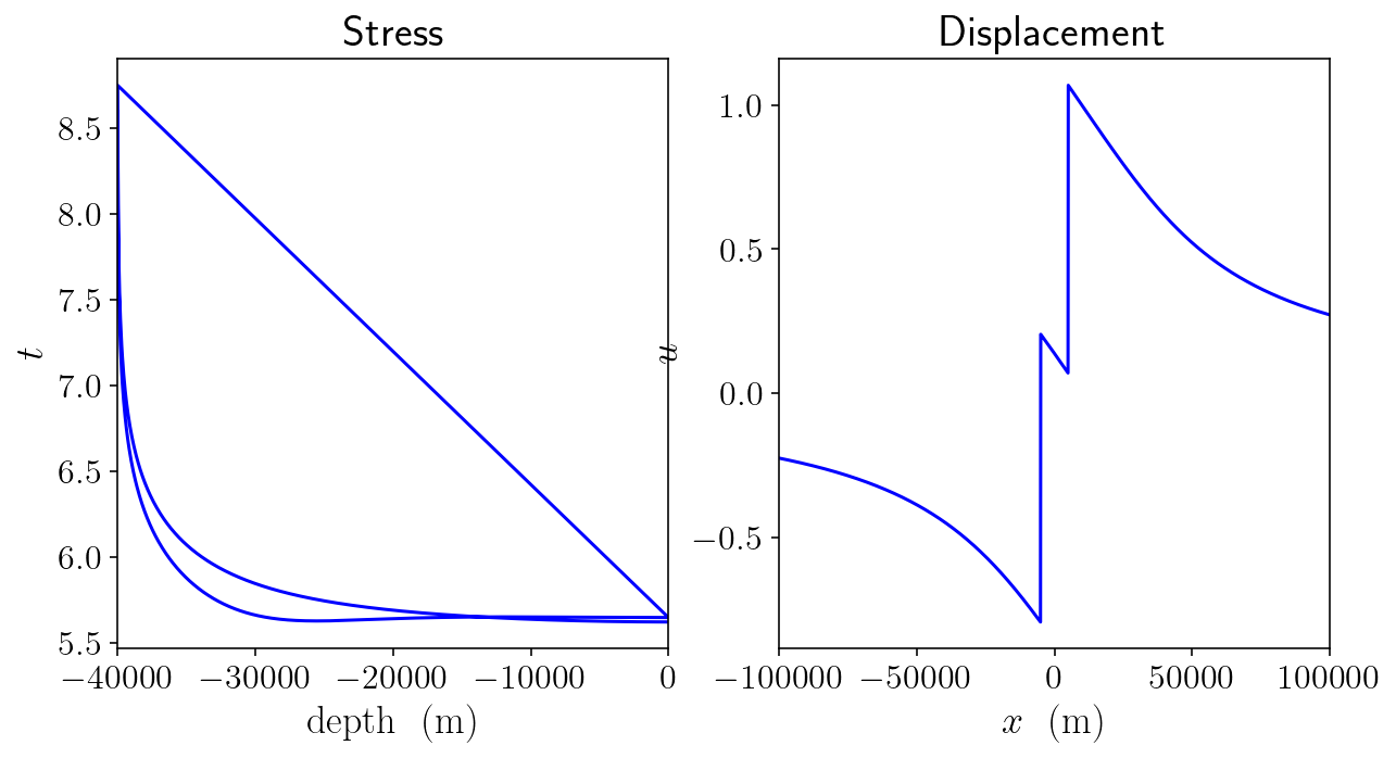
A = -fault_slip_to_fault_traction
B = -free_disp_to_fault_traction
C = fault_slip_to_free_disp
Dinv = np.linalg.inv(free_disp_solve_mat)

total_fault_slip_to_fault_traction = A - B.dot(Dinv.dot(C))
analytical_sd = -np.arctan(-fault_bottom / free.pts[:,0]) / np.pi
numerical_sd = Dinv.dot(-C).sum(axis=1)
rp = (faults.pts[:,1] + 1) ** 2
analytical_ft = -(shear_modulus / (2 * np.pi)) * ((1.0 / (faults.pts[:,1] + fault_bottom)) - (1.0 / (faults.pts[:,1] - fault_bottom)))
numerical_ft = total_fault_slip_to_fault_traction.sum(axis=1)
plt.figure(figsize=(10,5))
plt.subplot(1,2,1)
plt.title('Stress')
plt.plot(faults.pts[:,1], np.log10(np.abs(numerical_ft)), 'b-')
plt.xlim([-fault_bottom, 0])
plt.xlabel('$\mathrm{depth ~~ (m)}$')
plt.ylabel('$t$')
plt.subplot(1,2,2)
plt.title('Displacement')
plt.plot(free.pts[:,0], numerical_sd, 'b-')
plt.xlim([-100000, 100000])
plt.xlabel('$x ~~ \mathrm{(m)}$')
plt.ylabel('$u$')
plt.show()
7.3. Rate and state friction
siay = 31556952 # seconds in a year
density = 2670 # rock density (kg/m^3)
cs = np.sqrt(shear_modulus / density) # Shear wave speed (m/s)
eta = shear_modulus / (2 * cs) # The radiation damping coefficient (kg / (m^2 * s))
Vp = 1e-9 # Rate of plate motion
sigma_n = 50e6 # Normal stress (Pa)
# parameters describing "a", the coefficient of the direct velocity strengthening effect
a0 = 0.01
amax = 0.025
fy = faults.pts[:, 1]
H = 15000
h = 3000
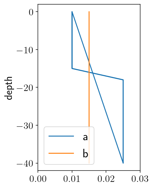
fp_a = np.where(
fy > -H, a0, np.where(fy > -(H + h), a0 + (amax - a0) * (fy + H) / -h, amax)
)
# state-based velocity weakening effect
fp_b = 0.015
# state evolution length scale (m)
fp_Dc = 0.008
# baseline coefficient of friction
fp_f0 = 0.6
# if V = V0 and at steady state, then f = f0, units are m/s
fp_V0 = 1e-6
plt.figure(figsize=(3, 5))
plt.plot(fp_a, fy/1000, label='a')
plt.plot(np.full(fy.shape[0], fp_b), fy/1000, label='b')
plt.xlim([0, 0.03])
plt.ylabel('depth')
plt.legend()
plt.show()
# The regularized form of the aging law.
def aging_law(fp_a, V, state):
    return (fp_b * fp_V0 / fp_Dc) * (np.exp((fp_f0 - state) / fp_b) - (V / fp_V0))

def qd_equation(fp_a, shear_stress, V, state):
    # The regularized rate and state friction equation
    F = sigma_n * fp_a * np.arcsinh(V / (2 * fp_V0) * np.exp(state / fp_a))

    # The full shear stress balance:
    return shear_stress - eta * V - F

def qd_equation_dV(fp_a, V, state):
    # First calculate the derivative of the friction law with respect to velocity
    # This is helpful for equation solving using Newton's method
    expsa = np.exp(state / fp_a)
    Q = (V * expsa) / (2 * fp_V0)
    dFdV = fp_a * expsa * sigma_n / (2 * fp_V0 * np.sqrt(1 + Q * Q))

    # The derivative of the full shear stress balance.
    return -eta - dFdV


def solve_friction(fp_a, shear, V_old, state, tol=1e-10):
    V = V_old
    max_iter = 150
    for i in range(max_iter):
        # Newton's method step!
        f = qd_equation(fp_a, shear, V, state)
        dfdv = qd_equation_dV(fp_a, V, state)
        step = f / dfdv

        # We know that slip velocity should not be negative so any step that
        # would lead to negative slip velocities is "bad". In those cases, we
        # cut the step size in half iteratively until the step is no longer
        # bad. This is a backtracking line search.
        while True:
            bad = step > V
            if np.any(bad):
                step[bad] *= 0.5
            else:
                break

        # Take the step and check if everything has converged.
        Vn = V - step
        if np.max(np.abs(step) / Vn) < tol:
            break
        V = Vn
        if i == max_iter - 1:
            raise Exception("Failed to converge.")

    # Return the solution and the number of iterations required.
    return Vn, i
for fm in [fault1, fault2]:
    mesh_L = np.max(np.abs(np.diff(fm.pts[:, 1])))
    Lb = shear_modulus * fp_Dc / (sigma_n * fp_b)
    hstar = (np.pi * shear_modulus * fp_Dc) / (sigma_n * (fp_b - fp_a))
    print(mesh_L, Lb, np.min(hstar[hstar > 0]))
53.84693101057201 341.3333333333333 3216.990877275949
53.84693101057201 341.3333333333333 3216.990877275949
7.4. Quasidynamic earthquake cycle derivatives
from scipy.optimize import fsolve
import copy

init_state_scalar = fsolve(lambda S: aging_law(fp_a, Vp, S), 0.7)[0]
init_state = np.full(faults.n_pts, init_state_scalar)
tau_amax = -qd_equation(amax, 0, Vp, init_state_scalar)

init_traction = np.full(faults.n_pts, tau_amax)
init_slip_deficit = np.zeros(faults.n_pts)
init_conditions = np.concatenate((init_slip_deficit, init_state))
class SystemState:

    V_old = np.full(faults.n_pts, Vp)
    state = None

    def calc(self, t, y, verbose=False):
        # Separate the slip_deficit and state sub components of the
        # time integration state.
        slip_deficit = y[: init_slip_deficit.shape[0]]
        state = y[init_slip_deficit.shape[0] :]

        # If the state values are bad, then the adaptive integrator probably
        # took a bad step.
        if np.any((state < 0) | (state > 2.0)):
            return False

        # The big three lines solving for quasistatic shear stress, slip rate
        # and state evolution
        tau_qs = init_traction - total_fault_slip_to_fault_traction.dot(slip_deficit)
        V = solve_friction(fp_a, tau_qs, self.V_old, state)[0]
        dstatedt = aging_law(fp_a, V, state)
        if not np.all(np.isfinite(V)):
            return False
        self.V_old = V

        slip_deficit_rate = Vp - V
        out = slip_deficit, state, tau_qs, V, slip_deficit_rate, dstatedt
        self.state = out
        return self.state


def plot_system_state(SS):
    """This is just a helper function that creates some rough plots of the
    current state to help with debugging"""
    slip_deficit, state, tau_qs, slip_deficit_rate, dstatedt = SS

    plt.figure(figsize=(15, 9))
    plt.subplot(2, 3, 1)
    plt.title("slip")
    plt.plot(faults.pts[:, 1], slip_deficit)

    plt.subplot(2, 3, 2)
    plt.title("state")
    plt.plot(faults.pts[:, 1], state)

    plt.subplot(2, 3, 3)
    plt.title("tau qs")
    plt.plot(faults.pts[:, 1], tau_qs)

    plt.subplot(2, 3, 4)
    plt.title("slip rate")
    plt.plot(faults.pts[:, 1], slip_deficit_rate)

    plt.subplot(2, 3, 6)
    plt.title("dstatedt")
    plt.plot(faults.pts[:, 1], dstatedt)
    plt.tight_layout()

    plt.show()


def calc_derivatives(state, t, y):
    """
    This helper function calculates the system state and then extracts the
    relevant derivatives that the integrator needs. It also intentionally
    returns infinite derivatives when the `y` vector provided by the integrator
    is invalid.
    """
    if not np.all(np.isfinite(y)):
        return np.inf * y
    state = state.calc(t, y)
    if not state:
        return np.inf * y
    derivatives = np.concatenate((state[-2], state[-1]))
    return derivatives
7.5. Integrating through time
%%time
from scipy.integrate import RK45

# We use a 5th order adaptive Runge Kutta method and pass the derivative function to it
# the relative tolerance will be 1e-11 to make sure that even
state = SystemState()
derivs = lambda t, y: calc_derivatives(state, t, y)
integrator = RK45
atol = Vp * 1e-6
rtol = 1e-11
rk = integrator(derivs, 0, init_conditions, 1e50, atol=atol, rtol=rtol)

# Set the initial time step to one day.
rk.h_abs = 60 * 60 * 24

# Integrate for 1000 years.
max_T = 1000 * siay

n_steps = 1000000
t_history = [0]
y_history = [init_conditions.copy()]
for i in range(n_steps):

    # Take a time step and store the result
    if rk.step() != None:
        raise Exception("TIME STEPPING FAILED")
        break
    t_history.append(rk.t)
    y_history.append(rk.y.copy())

    # Print the time every 5000 steps
    if i % 5000 == 0:
        print(f"step={i}, time={rk.t / siay} yrs, step={(rk.t - t_history[-2]) / siay}")
    if rk.t > max_T:
        break

y_history = np.array(y_history)
t_history = np.array(t_history)
step=0, time=0.002737907006988508 yrs, step=0.002737907006988508
step=5000, time=161.2388012289919 yrs, step=6.068323795478569e-11
step=10000, time=161.238801483585 yrs, step=3.200375945922213e-11
step=15000, time=177.06735503165402 yrs, step=0.05782401363757997
step=20000, time=187.60702659014385 yrs, step=8.29256996752649e-11
step=25000, time=187.6070269264095 yrs, step=2.786049654906221e-10
step=30000, time=213.4153146695212 yrs, step=1.3348499105890855e-10
step=35000, time=229.49165911338014 yrs, step=1.8458825569115088e-10
step=40000, time=298.5155537603046 yrs, step=1.1030568652139828e-10
step=45000, time=298.51555399934733 yrs, step=3.251751197178755e-11
step=50000, time=298.5168884817506 yrs, step=6.51359998844683e-06
step=55000, time=323.01280183052285 yrs, step=1.2281707123916784e-10
step=60000, time=323.01280207887106 yrs, step=3.3484575524851865e-11
step=65000, time=323.2817940109216 yrs, step=0.001729718400292269
step=70000, time=351.52626665410605 yrs, step=1.0785478482910092e-08
step=75000, time=368.9516542294202 yrs, step=1.2976784052681758e-10
step=80000, time=368.951654876993 yrs, step=6.515590688770813e-11
step=85000, time=428.9915445603336 yrs, step=0.0014206634043130257
step=90000, time=446.2939275656298 yrs, step=6.588120455250637e-11
step=95000, time=446.29392801977554 yrs, step=9.456068304806992e-10
step=100000, time=469.8994523682489 yrs, step=1.0256917809688377e-10
step=105000, time=469.89945268723017 yrs, step=5.1798341561007304e-11
step=110000, time=469.9812354270467 yrs, step=0.00034767164051762437
step=115000, time=500.90614938849876 yrs, step=1.439715864624497e-10
step=120000, time=573.9064649517662 yrs, step=1.424001081887202e-10
step=125000, time=573.9064651906277 yrs, step=2.5022769435539118e-11
step=130000, time=597.5674917048766 yrs, step=0.0012973735857483035
step=135000, time=597.6230358626846 yrs, step=5.391379308333549e-11
step=140000, time=597.6230366893858 yrs, step=4.587749495737104e-09
step=145000, time=625.2112327038584 yrs, step=1.1906969997104363e-10
step=150000, time=642.3455004578122 yrs, step=1.2898210138995284e-10
step=155000, time=704.8417989867936 yrs, step=0.003113930973116129
step=160000, time=716.3612963754118 yrs, step=2.9978970144993726e-11
step=165000, time=716.3612966987445 yrs, step=3.9843018386249724e-10
step=170000, time=743.0069768079197 yrs, step=1.6222491102653862e-10
step=175000, time=743.0069772376432 yrs, step=4.6660816435353134e-11
step=180000, time=743.0070823319467 yrs, step=6.836717438689674e-07
step=185000, time=772.4229461837367 yrs, step=1.1205848921132735e-10
step=190000, time=790.5550252030326 yrs, step=9.598105764163313e-11
step=195000, time=790.5550257931098 yrs, step=9.694812119469745e-11
step=200000, time=790.5770082962302 yrs, step=0.00011880289499414454
step=205000, time=843.4093589520743 yrs, step=1.3986156636192637e-10
step=210000, time=843.4093595399053 yrs, step=5.7540281407326665e-11
step=215000, time=865.8601485323139 yrs, step=4.5113514750450234e-10
step=220000, time=903.1263077569464 yrs, step=1.2438854951289735e-10
step=225000, time=903.1263082887026 yrs, step=8.413452911659529e-11
step=230000, time=927.4523165504868 yrs, step=0.008045238903279458
step=235000, time=947.0642174585033 yrs, step=1.7528026899290684e-11
step=240000, time=947.0685830652857 yrs, step=1.768826485736451e-05
step=245000, time=972.5636479272499 yrs, step=4.078590535048743e-10
step=250000, time=988.09794803525 yrs, step=8.195863612220059e-11
step=255000, time=988.0979484325295 yrs, step=2.7077779485800782e-11
CPU times: user 2h 15min 3s, sys: 36min 52s, total: 2h 51min 55s
Wall time: 1h 48min 42s
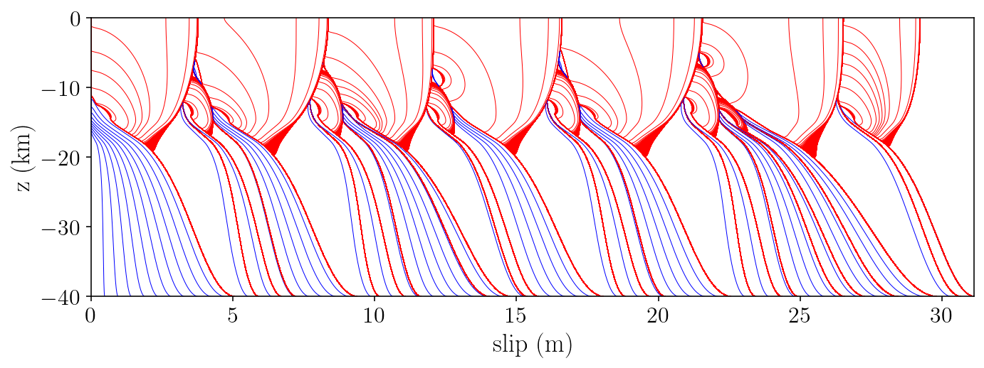
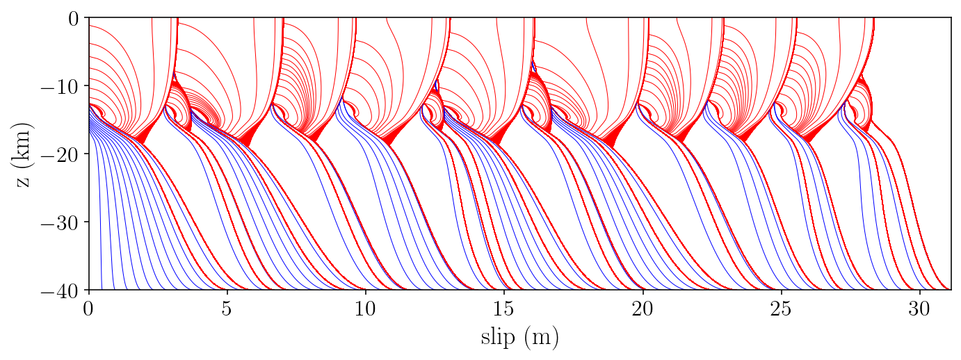
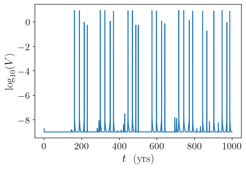
7.6. Plotting the results
derivs_history = np.diff(y_history, axis=0) / np.diff(t_history)[:, None]
max_vel = np.max(np.abs(derivs_history), axis=1)
plt.plot(t_history[1:] / siay, np.log10(max_vel))
plt.xlabel('$t ~~ \mathrm{(yrs)}$')
plt.ylabel('$\log_{10}(V)$')
plt.show()
for j in range(2):
    fm = fault1 if j == 0 else fault2
    plt.figure(figsize=(10, 4))
    last_plt_t = -1000
    last_plt_slip = init_slip_deficit
    event_times = []
    for i in range(len(y_history) - 1):
        y = y_history[i]
        t = t_history[i]
        slip_deficit_full = y[: init_slip_deficit.shape[0]]
        fault1_sd = slip_deficit_full[:fault1.n_pts]
        fault2_sd = slip_deficit_full[fault1.n_pts:]
        slip_deficit = fault1_sd if j == 0 else fault2_sd
        should_plot = False

        # Plot a red line every three second if the slip rate is over 0.1 mm/s.
        if (
            max_vel[i] >= 0.0001 and t - last_plt_t > 3
        ):
            if len(event_times) == 0 or t - event_times[-1] > siay:
                event_times.append(t)
            should_plot = True
            color = "r"

        # Plot a blue line every fifteen years during the interseismic period
        if t - last_plt_t > 15 * siay:
            should_plot = True
            color = "b"

        if should_plot:
            # Convert from slip deficit to slip:
            slip = -slip_deficit + Vp * t
            plt.plot(slip, fm.pts[:,1] / 1000.0, color + "-", linewidth=0.5)
            last_plt_t = t
            last_plt_slip = slip
    plt.xlim([0, np.max(last_plt_slip)])
    plt.ylim([-40, 0])
    plt.ylabel(r"$\textrm{z (km)}$")
    plt.xlabel(r"$\textrm{slip (m)}$")
    plt.tight_layout()
    plt.savefig("halfspace.png", dpi=300)
    plt.show()