8. [DRAFT] Quasidynamic thrust fault earthquake cycles (plane strain)¶

8.1. Summary¶

Most of the code here follows almost exactly from the previous section on strike-slip/antiplane earthquake cycles.
Since the fault motion is in the same plane as the fault normal vectors, we are no longer operating in an antiplane approximation. Instead, we use plane strain elasticity, a different 2D reduction of full 3D elasticity.
One key difference is the vector nature of the displacement and the tensor nature of the stress. We must always make sure we are dealing with tractions on the correct surface.
We construct a mesh, build our discrete boundary integral operators, step through time and then compare against other benchmark participants’ results.

Does this section need detailed explanation or is it best left as lonely code? Most of the explanation would be redundant with the antiplane QD document.

import sympy as sp
import numpy as np
import matplotlib.pyplot as plt
from tectosaur2 import gauss_rule, refine_surfaces, integrate_term, panelize_symbolic_surface
from tectosaur2.elastic2d import elastic_t, elastic_h
from tectosaur2.rate_state import MaterialProps, qd_equation, solve_friction, aging_law

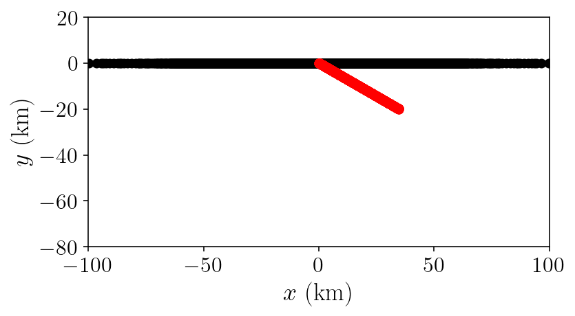
surf_half_L = 1000000
fault_length = 40000
max_panel_length = 400
n_fault = 400
mu = shear_modulus = 3.2e10
nu = 0.25

quad_rule = gauss_rule(6)
sp_t = sp.var("t")

angle_rad = sp.pi / 6
sp_x = (sp_t + 1) / 2 * sp.cos(angle_rad) * fault_length
sp_y = -(sp_t + 1) / 2 * sp.sin(angle_rad) * fault_length
fault = panelize_symbolic_surface(
    sp_t, sp_x, sp_y,
    quad_rule,
    n_panels=n_fault
)

free = refine_surfaces(
    [
        (sp_t, -sp_t * surf_half_L, 0 * sp_t)  # free surface
    ],
    quad_rule,
    control_points = [
        # nearfield surface panels and fault panels will be limited to 200m
        # at 200m per panel, we have ~40m per solution node because the panels
        # have 5 nodes each
        (0, 0, 1.5 * fault_length, max_panel_length),
        (0, 0, 0.2 * fault_length, 1.5 * fault_length / (n_fault)),
        # farfield panels will be limited to 200000 m per panel at most
        (0, 0, surf_half_L, 50000),
    ]
)
print(
    f"The free surface mesh has {free.n_panels} panels with a total of {free.n_pts} points."
)
print(
    f"The fault mesh has {fault.n_panels} panels with a total of {fault.n_pts} points."
)

The free surface mesh has 646 panels with a total of 3876 points.
The fault mesh has 400 panels with a total of 2400 points.

plt.plot(free.pts[:,0]/1000, free.pts[:,1]/1000, 'k-o')
plt.plot(fault.pts[:,0]/1000, fault.pts[:,1]/1000, 'r-o')
plt.xlabel(r'$x ~ \mathrm{(km)}$')
plt.ylabel(r'$y ~ \mathrm{(km)}$')
plt.axis('scaled')
plt.xlim([-100, 100])
plt.ylim([-80, 20])
plt.show()

And, to start off the integration, we’ll construct the operators necessary for solving for free surface displacement from fault slip.

singularities = np.array(
    [
        [-surf_half_L, 0],
        [surf_half_L, 0],
        [0, 0],
        [float(sp_x.subs(sp_t,1)), float(sp_y.subs(sp_t,1))],
    ]
)

(free_disp_to_free_disp, fault_slip_to_free_disp), report = integrate_term(
    elastic_t(nu), free.pts, free, fault, singularities=singularities, safety_mode=True, return_report=True
)

/Users/tbent/Dropbox/active/eq/tectosaur2/tectosaur2/integrate.py:204: UserWarning: Some integrals failed to converge during adaptive integration. This an indication of a problem in either the integration or the problem formulation.
  warnings.warn(

fault_slip_to_free_disp = fault_slip_to_free_disp.reshape((-1, 2 * fault.n_pts))
free_disp_to_free_disp = free_disp_to_free_disp.reshape((-1, 2 * free.n_pts))
free_disp_solve_mat = (
    np.eye(free_disp_to_free_disp.shape[0]) + free_disp_to_free_disp
)

from tectosaur2.elastic2d import ElasticH

(free_disp_to_fault_stress, fault_slip_to_fault_stress), report = integrate_term(
    ElasticH(nu, d_cutoff=8.0),
    # elastic_h(nu),
    fault.pts,
    free,
    fault,
    tol=1e-12,
    safety_mode=True,
    singularities=singularities,
    return_report=True,
)
fault_slip_to_fault_stress *= shear_modulus
free_disp_to_fault_stress *= shear_modulus

We’re not achieving the tolerance we asked for!! Hypersingular integrals can be tricky but I think this is solvable.

report['integration_error'].max()

1.4504879515499894e-07

A = -fault_slip_to_fault_stress.reshape((-1, 2 * fault.n_pts))
B = -free_disp_to_fault_stress.reshape((-1, 2 * free.n_pts))
C = fault_slip_to_free_disp
Dinv = np.linalg.inv(free_disp_solve_mat)
total_fault_slip_to_fault_stress = A - B.dot(Dinv.dot(C))

nx = fault.normals[:, 0]
ny = fault.normals[:, 1]
normal_mult = np.transpose(np.array([[nx, 0 * nx, ny], [0 * nx, ny, nx]]), (2, 0, 1))

total_fault_slip_to_fault_traction = np.sum(
    total_fault_slip_to_fault_stress.reshape((-1, 3, fault.n_pts, 2))[:, None, :, :, :]
    * normal_mult[:, :, :, None, None],
    axis=2,
).reshape((-1, 2 * fault.n_pts))

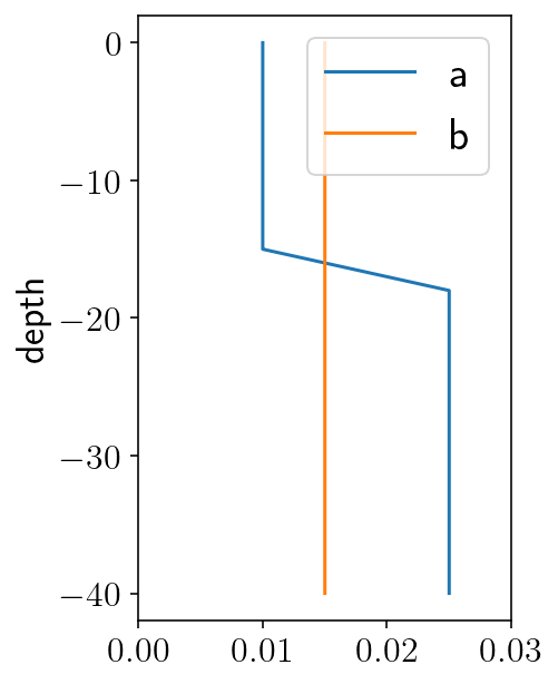
8.2. Rate and state friction¶

siay = 31556952  # seconds in a year
density = 2670  # rock density (kg/m^3)
cs = np.sqrt(shear_modulus / density)  # Shear wave speed (m/s)
Vp = 1e-9  # Rate of plate motion
sigma_n0 = 50e6  # Normal stress (Pa)

# parameters describing "a", the coefficient of the direct velocity strengthening effect
a0 = 0.01
amax = 0.025
H = 15000
h = 3000
fx = fault.pts[:, 0]
fy = fault.pts[:, 1]
fd = -np.sqrt(fx ** 2 + fy ** 2)
a = np.where(
    fd > -H, a0, np.where(fd > -(H + h), a0 + (amax - a0) * (fd + H) / -h, amax)
)

mp = MaterialProps(a=a, b=0.015, Dc=0.008, f0=0.6, V0=1e-6, eta=shear_modulus / (2 * cs))

plt.figure(figsize=(3, 5))
plt.plot(mp.a, fd/1000, label='a')
plt.plot(np.full(fy.shape[0], mp.b), fd/1000, label='b')
plt.xlim([0, 0.03])
plt.ylabel('depth')
plt.legend()
plt.show()

mesh_L = np.max(np.abs(np.diff(fd)))
Lb = shear_modulus * mp.Dc / (sigma_n0 * mp.b)
hstar = (np.pi * shear_modulus * mp.Dc) / (sigma_n0 * (mp.b - mp.a))
mesh_L, Lb, np.min(hstar[hstar > 0])

(23.861918608330598, 341.3333333333333, 3216.990877275949)

8.3. Quasidynamic earthquake cycle derivatives¶

from scipy.optimize import fsolve
import copy

init_state_scalar = fsolve(lambda S: aging_law(mp, Vp, S), 0.7)[0]
mp_amax = copy.copy(mp)
mp_amax.a=amax
tau_amax = -qd_equation(mp_amax, sigma_n0, 0, Vp, init_state_scalar)
init_state = np.log((2*mp.V0/Vp)*np.sinh((tau_amax - mp.eta*Vp) / (mp.a*sigma_n0))) * mp.a

init_tau = np.full(fault.n_pts, tau_amax)
init_sigma = np.full(fault.n_pts, sigma_n0)
init_slip_deficit = np.zeros(fault.n_pts)
init_conditions = np.concatenate((init_slip_deficit, init_state))

class SystemState:

    V_old = np.full(fault.n_pts, Vp)
    state = None

    def calc(self, t, y, verbose=False):
        # Separate the slip_deficit and state sub components of the
        # time integration state.
        slip_deficit = y[: init_slip_deficit.shape[0]]
        state = y[init_slip_deficit.shape[0] :]

        # If the state values are bad, then the adaptive integrator probably
        # took a bad step.
        if np.any((state < 0) | (state > 2.0)):
            print("bad state")
            return False

        # The big three lines solving for quasistatic shear stress, slip rate
        # and state evolution
        sd_vector = np.stack((slip_deficit * -ny, slip_deficit * nx), axis=1).ravel()
        traction = total_fault_slip_to_fault_traction.dot(sd_vector).reshape((-1, 2))
        delta_sigma_qs = np.sum(traction * np.stack((nx, ny), axis=1), axis=1)
        delta_tau_qs = -np.sum(traction * np.stack((-ny, nx), axis=1), axis=1)
        tau_qs = init_tau + delta_tau_qs
        sigma_qs = init_sigma + delta_sigma_qs

        V = solve_friction(mp, sigma_qs, tau_qs, self.V_old, state)
        if not V[2]:
            print("convergence failed")
            return False

        V=V[0]
        if not np.all(np.isfinite(V)):
            print("infinite V")
            return False
        dstatedt = aging_law(mp, V, state)
        self.V_old = V

        slip_deficit_rate = Vp - V
        out = (
            slip_deficit,
            state,
            delta_sigma_qs,
            sigma_qs,
            delta_tau_qs,
            tau_qs,
            V,
            slip_deficit_rate,
            dstatedt,
        )
        self.data = out
        return self.data

def plot_system_state(t, SS, xlim=None):
    """This is just a helper function that creates some rough plots of the
    current state to help with debugging"""
    (
        slip_deficit,
        state,
        delta_sigma_qs,
        sigma_qs,
        delta_tau_qs,
        tau_qs,
        V,
        slip_deficit_rate,
        dstatedt,
    ) = SS

    slip = Vp * t - slip_deficit

    fd = -np.linalg.norm(fault.pts, axis=1)

    plt.figure(figsize=(15, 9))
    plt.suptitle(f"t={t/siay}")
    plt.subplot(3, 3, 1)
    plt.title("slip")
    plt.plot(fd, slip)
    plt.xlim(xlim)

    plt.subplot(3, 3, 2)
    plt.title("slip deficit")
    plt.plot(fd, slip_deficit)
    plt.xlim(xlim)

    # plt.subplot(3, 3, 2)
    # plt.title("slip deficit rate")
    # plt.plot(fd, slip_deficit_rate)
    # plt.xlim(xlim)

    # plt.subplot(3, 3, 2)
    # plt.title("strength")
    # plt.plot(fd, tau_qs/sigma_qs)
    # plt.xlim(xlim)

    plt.subplot(3, 3, 3)
    # plt.title("log V")
    # plt.plot(fd, np.log10(V))
    plt.title("V")
    plt.plot(fd, V)
    plt.xlim(xlim)

    plt.subplot(3, 3, 4)
    plt.title(r"$\sigma_{qs}$")
    plt.plot(fd, sigma_qs)
    plt.xlim(xlim)

    plt.subplot(3, 3, 5)
    plt.title(r"$\tau_{qs}$")
    plt.plot(fd, tau_qs, 'k-o')
    plt.xlim(xlim)

    plt.subplot(3, 3, 6)
    plt.title("state")
    plt.plot(fd, state)
    plt.xlim(xlim)

    plt.subplot(3, 3, 7)
    plt.title(r"$\Delta\sigma_{qs}$")
    plt.plot(fd, delta_sigma_qs)
    plt.hlines([0], [fd[-1]], [fd[0]])
    plt.xlim(xlim)

    plt.subplot(3, 3, 8)
    plt.title(r"$\Delta\tau_{qs}$")
    plt.plot(fd, delta_tau_qs)
    plt.hlines([0], [fd[-1]], [fd[0]])
    plt.xlim(xlim)

    plt.subplot(3, 3, 9)
    plt.title("dstatedt")
    plt.plot(fd, dstatedt)
    plt.xlim(xlim)
    plt.tight_layout()

    plt.show()

def calc_derivatives(state, t, y):
    """
    This helper function calculates the system state and then extracts the
    relevant derivatives that the integrator needs. It also intentionally
    returns infinite derivatives when the `y` vector provided by the integrator
    is invalid.
    """
    if not np.all(np.isfinite(y)):
        return np.inf * y
    state_vecs = state.calc(t, y)
    if not state_vecs:
        return np.inf * y
    derivatives = np.concatenate((state_vecs[-2], state_vecs[-1]))
    return derivatives

8.4. Integrating through time¶

%%time
from scipy.integrate import RK23, RK45

# We use a 5th order adaptive Runge Kutta method and pass the derivative function to it
# the relative tolerance will be 1e-11 to make sure that even
state = SystemState()
derivs = lambda t, y: calc_derivatives(state, t, y)
integrator = RK45
atol = Vp * 1e-6
rtol = 1e-11
rk = integrator(derivs, 0, init_conditions, 1e50, atol=atol, rtol=rtol)

# Set the initial time step to one day.
rk.h_abs = 60 * 60 * 24

# Integrate for 1000 years.
max_T = 1000 * siay

n_steps = 500000
t_history = [0]
y_history = [init_conditions.copy()]
for i in range(n_steps):
    # Take a time step and store the result
    if rk.step() != None:
        raise Exception("TIME STEPPING FAILED")
    t_history.append(rk.t)
    y_history.append(rk.y.copy())

    # Print the time every 5000 steps
    if i % 5000 == 0:
        print(f"step={i}, time={rk.t / siay} yrs, step={(rk.t - t_history[-2]) / siay}")

    if rk.t > max_T:
        break

y_history = np.array(y_history)
t_history = np.array(t_history)

step=0, time=1.4616397558414107e-05 yrs, step=1.4616397558414107e-05
step=5000, time=133.40079223999558 yrs, step=0.025598497379265003
step=10000, time=176.14015294812103 yrs, step=5.998816102602071e-11
step=15000, time=176.14015339898557 yrs, step=8.238172642666623e-11
step=20000, time=176.14296040288025 yrs, step=2.1979783596630634e-05
step=25000, time=263.1375647457368 yrs, step=0.0006967333900754272
step=30000, time=263.2373556060858 yrs, step=5.5787478717397596e-11
step=35000, time=263.23735589847996 yrs, step=1.6116718526537453e-10
step=40000, time=314.8023513177958 yrs, step=0.030260419123390083
step=45000, time=327.9773806823734 yrs, step=7.065608084576142e-11
step=50000, time=327.97738099773073 yrs, step=3.294060227625318e-11
step=55000, time=356.3693505901927 yrs, step=0.02798904784696968
step=60000, time=414.56802731019104 yrs, step=4.732567262808485e-11
step=65000, time=414.56802756651166 yrs, step=4.1885940142098087e-11
step=70000, time=414.9294840754991 yrs, step=0.002112030610137971
step=75000, time=479.28663934235965 yrs, step=5.784248876765926e-11
step=80000, time=479.28663967884637 yrs, step=7.796949896581029e-11
step=85000, time=479.2877011529307 yrs, step=8.501305135281465e-06
step=90000, time=565.6498981880231 yrs, step=0.001480316487609428
step=95000, time=565.8770021991605 yrs, step=5.4639090748133724e-11
step=100000, time=565.877002481205 yrs, step=1.531586902165607e-10
step=105000, time=614.5975778365752 yrs, step=0.029474945371490282
step=110000, time=630.595404186933 yrs, step=6.22547162285152e-11
step=115000, time=630.5954045063037 yrs, step=3.6990180904709996e-11
step=120000, time=656.0166350083252 yrs, step=0.02921588740701827
step=125000, time=717.1857705022477 yrs, step=4.0979318061100294e-11
step=130000, time=717.1857707585524 yrs, step=5.234231480960598e-11
step=135000, time=717.3785763542687 yrs, step=0.0010220541964367556
step=140000, time=781.904169712801 yrs, step=6.805709754690108e-11
step=145000, time=781.904170048407 yrs, step=7.603537185968166e-11
step=150000, time=781.9045694275084 yrs, step=3.6081749206038533e-06
step=155000, time=867.9930534924584 yrs, step=0.0034391542903144255
step=160000, time=868.4945363826215 yrs, step=5.258408069787206e-11
step=165000, time=868.4945366547215 yrs, step=1.5182897783109724e-10
step=170000, time=914.161314434437 yrs, step=0.030127968410185897
step=175000, time=933.2129355866244 yrs, step=7.228800059155745e-11
step=180000, time=933.2129359097105 yrs, step=3.505605379858137e-11
step=185000, time=955.611410869588 yrs, step=0.025085701504597362
CPU times: user 5h 6min 33s, sys: 27min 1s, total: 5h 33min 35s
Wall time: 1h 27min 50s

8.5. Plotting the results¶

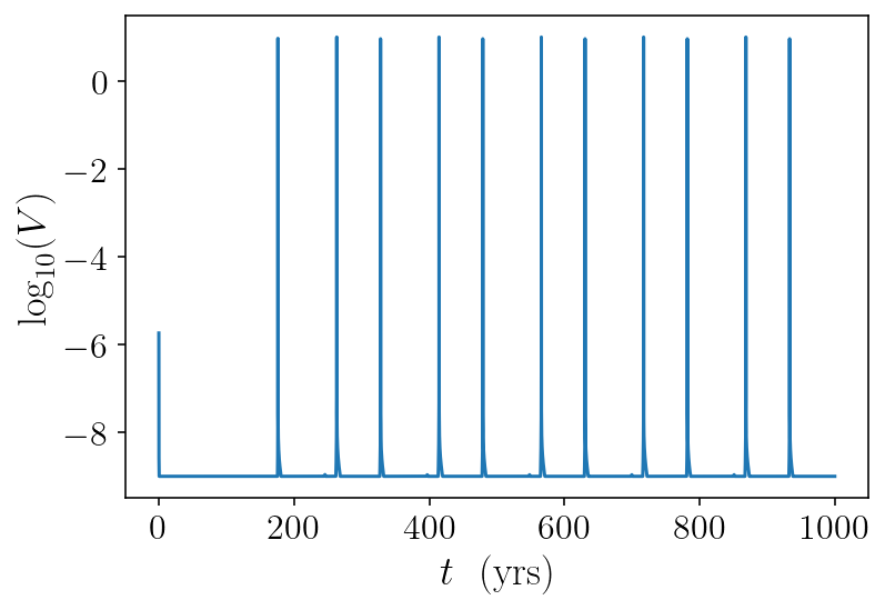
Now that we’ve solved for 1000 years of fault slip evolution, let’s plot some of the results. I’ll start with a super simple plot of the maximum log slip rate over time.

derivs_history = np.diff(y_history, axis=0) / np.diff(t_history)[:, None]
max_vel = np.max(np.abs(derivs_history), axis=1)
plt.plot(t_history[1:] / siay, np.log10(max_vel))
plt.xlabel('$t ~~ \mathrm{(yrs)}$')
plt.ylabel('$\log_{10}(V)$')
plt.show()

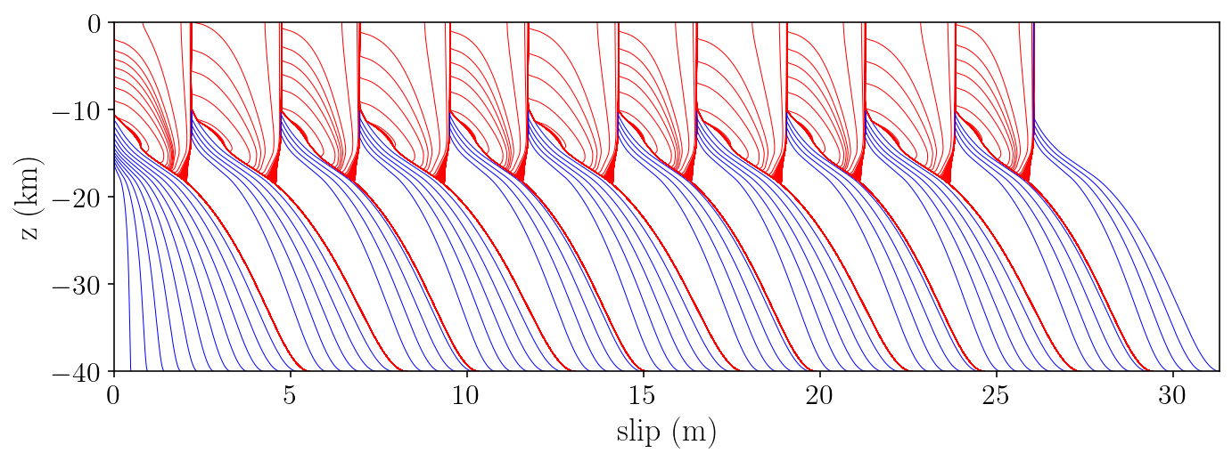
And next, we’ll make the classic plot showing the spatial distribution of slip over time:

the blue lines show interseismic slip evolution and are plotted every fifteen years
the red lines show evolution during rupture every three seconds.

plt.figure(figsize=(10, 4))
last_plt_t = -1000
last_plt_slip = init_slip_deficit
event_times = []
for i in range(len(y_history) - 1):
    y = y_history[i]
    t = t_history[i]
    slip_deficit = y[: init_slip_deficit.shape[0]]
    should_plot = False

    # Plot a red line every three second if the slip rate is over 0.1 mm/s.
    if (
        max_vel[i] >= 0.0001 and t - last_plt_t > 3
    ):
        if len(event_times) == 0 or t - event_times[-1] > siay:
            event_times.append(t)
        should_plot = True
        color = "r"

    # Plot a blue line every fifteen years during the interseismic period
    if t - last_plt_t > 15 * siay:
        should_plot = True
        color = "b"

    if should_plot:
        # Convert from slip deficit to slip:
        slip = -slip_deficit + Vp * t
        plt.plot(slip, fd / 1000.0, color + "-", linewidth=0.5)
        last_plt_t = t
        last_plt_slip = slip
plt.xlim([0, np.max(last_plt_slip)])
plt.ylim([-40, 0])
plt.ylabel(r"$\textrm{z (km)}$")
plt.xlabel(r"$\textrm{slip (m)}$")
plt.tight_layout()
plt.savefig("halfspace.png", dpi=300)
plt.show()

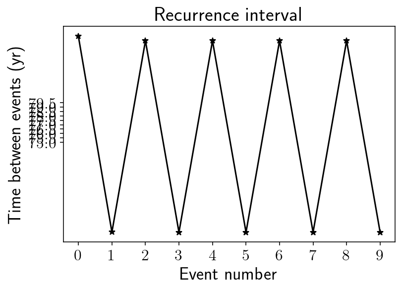
And a plot of recurrence interval:

plt.title("Recurrence interval")
plt.plot(np.diff(event_times) / siay, "k-*")
plt.xticks(np.arange(0, 10, 1))
plt.yticks(np.arange(75, 80, 0.5))
plt.xlabel("Event number")
plt.ylabel("Time between events (yr)")
plt.show()

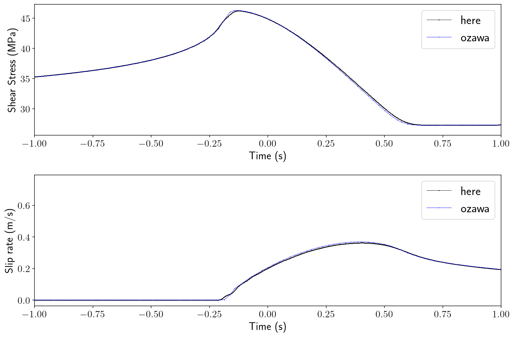
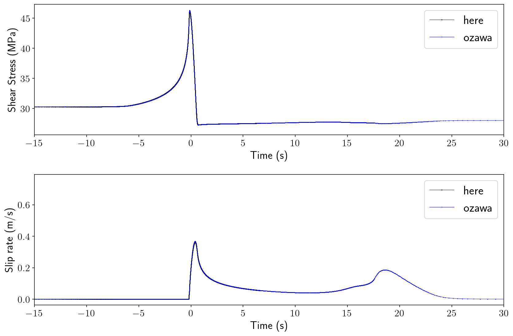
8.6. Comparison against SCEC SEAS results¶

ozawa_data = np.loadtxt("ozawa7500.txt")
ozawa_slip_rate = 10 ** ozawa_data[:, 2]
ozawa_stress = ozawa_data[:, 3]

t_start_idx = np.argmax(max_vel > 1e-4)
t_end_idx = np.argmax(max_vel[t_start_idx:] < 1e-6)
n_steps = t_end_idx - t_start_idx
t_chunk = t_history[t_start_idx : t_end_idx]

shear_chunk = []
slip_rate_chunk = []
for i in range(n_steps):
    system_state = SystemState().calc(t_history[t_start_idx + i], y_history[t_start_idx + i])
    slip_deficit, state, delta_sigma_qs, sigma_qs, delta_tau_qs, tau_qs, V, slip_deficit_rate, dstatedt = system_state
    shear_chunk.append((tau_qs - mp.eta * V))
    slip_rate_chunk.append(V)
shear_chunk = np.array(shear_chunk)
slip_rate_chunk = np.array(slip_rate_chunk)

fault_idx = np.argmax((-7450 > fd) & (fd > -7550))
VAvg = np.mean(slip_rate_chunk[:, fault_idx:(fault_idx+2)], axis=1)
SAvg = np.mean(shear_chunk[:, fault_idx:(fault_idx+2)], axis=1)

fault_idx

t_align = t_chunk[np.argmax(VAvg > 0.2)]
ozawa_t_align = np.argmax(ozawa_slip_rate > 0.2)

for lims in [(-1, 1), (-15, 30)]:
    plt.figure(figsize=(12, 8))
    plt.subplot(2, 1, 1)
    plt.plot(t_chunk - t_align, SAvg / 1e6, "k-o", markersize=0.5, linewidth=0.5, label='here')
    plt.plot(
        ozawa_data[:, 0] - ozawa_data[ozawa_t_align, 0],
        ozawa_stress,
        "b-*",
        markersize=0.5,
        linewidth=0.5,
        label='ozawa'
    )
    plt.legend()
    plt.xlim(lims)
    plt.xlabel("Time (s)")
    plt.ylabel("Shear Stress (MPa)")
    # plt.show()

    plt.subplot(2, 1, 2)
    plt.plot(t_chunk - t_align, VAvg, "k-o", markersize=0.5, linewidth=0.5, label='here')
    plt.plot(
        ozawa_data[:, 0] - ozawa_data[ozawa_t_align, 0],
        ozawa_slip_rate[:],
        "b-*",
        markersize=0.5,
        linewidth=0.5,
        label='ozawa'
    )
    plt.legend()
    plt.xlim(lims)
    plt.xlabel("Time (s)")
    plt.ylabel("Slip rate (m/s)")
    plt.tight_layout()
    plt.show()

Integral equation tutorials

[DRAFT] Quasidynamic thrust fault earthquake cycles (plane strain)

Contents