[DRAFT] Method of manufactured solutions (MMS) for the Poisson equation
Contents
2. [DRAFT] Method of manufactured solutions (MMS) for the Poisson equation
2.1. TODO:
The remaining fundamental issue is the singularity in the volume integral. Set up a way of testing the accuracy of this integral.
For the Poisson equation with Dirichlet boundary conditions:
\begin{split}
\nabla u &= f ~~ \textrm{in} ~~ \Omega\
u &= g ~~ \textrm{on} ~~ \partial \Omega
\end{split}
u_particular is the integral:
(2.5)¶\[\begin{equation}
v(x) = \int_{\Omega} G(x,y) f(y) dy
\end{equation}\]
which satisfies equation 1 but not 2.
Then, compute homogeneous solution, u_homog with appropriate boundary conditions:
\begin{split} \nabla u^H &= 0 ~~ \textrm{in} ~~ \Omega \ u^H &= g - v|_{\partial \Omega} ~~ \textrm{on} ~~ \partial \Omega \end{split}
So, first, I need to compute \(g - v|_{\partial \Omega}\)
2.2. Setup
import numpy as np
import matplotlib.pyplot as plt
import sympy as sp

from tectosaur2 import integrate_term, refine_surfaces, gauss_rule, trapezoidal_rule
from tectosaur2.laplace2d import single_layer, double_layer
nq = 10
quad_rule = gauss_rule(nq)

t = sp.symbols("t")
theta = sp.pi * (t + 1)
circle = refine_surfaces([(t, sp.cos(theta), sp.sin(theta))], quad_rule)
circle.n_pts, circle.n_panels
(320, 32)
x, y = sp.symbols('x, y')
sym_soln = 2 + x + y + x**2 + y*sp.cos(6*x) + x*sp.sin(6*y)

sym_laplacian = (
    sp.diff(sp.diff(sym_soln, x), x) +
    sp.diff(sp.diff(sym_soln, y), y)
)
soln_fnc = sp.lambdify((x, y), sym_soln, "numpy")
laplacian_fnc = sp.lambdify((x, y), sym_laplacian, "numpy")

sym_soln
\[\displaystyle x^{2} + x \sin{\left(6 y \right)} + x + y \cos{\left(6 x \right)} + y + 2\]
sym_laplacian
\[\displaystyle - 36 x \sin{\left(6 y \right)} - 36 y \cos{\left(6 x \right)} + 2\]
2.3. Body force quadrature
nq_r = 80
nq_theta = 160
qgauss, qgauss_w = gauss_rule(nq_r)[:2]
qtrap, qtrap_w = trapezoidal_rule(nq_theta)[:2]
r = 0.5 * (qgauss + 1)
r_w = qgauss_w * 0.5
theta = (qtrap + 1) * np.pi
theta_w = qtrap_w * np.pi

r_vol, theta_vol = [x.flatten() for x in np.meshgrid(r, theta)]
qx_vol = np.cos(theta_vol) * r_vol
qy_vol = np.sin(theta_vol) * r_vol

q2d_vol = np.array([qx_vol, qy_vol]).T.copy()
q2d_vol_wts = (r_w[None, :] * theta_w[:, None] * r[None, :]).flatten()
np.sum(q2d_vol_wts) - np.pi, np.sum(np.cos(theta_vol) * q2d_vol_wts), np.sum(r_vol * q2d_vol_wts) - 2.0943951023931954
(0.0, 0.0, 4.440892098500626e-16)
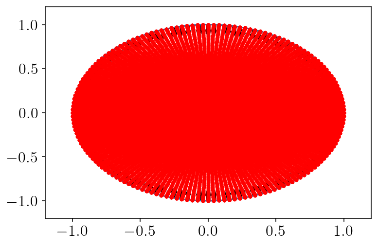
plt.plot(circle.pts[:, 0], circle.pts[:, 1])
plt.quiver(circle.pts[:, 0], circle.pts[:, 1], circle.normals[:, 0], circle.normals[:, 1])
plt.plot(q2d_vol[:, 0], q2d_vol[:, 1], "r.")
plt.xlim([-1.2, 1.2])
plt.ylim([-1.2, 1.2])
plt.show()
nobs = 200
offset = -0.1
zoomx = [-1.0 + offset, 1.0 - offset]
zoomy = [-1.0 + offset, 1.0 - offset]
xs = np.linspace(*zoomx, nobs)
ys = np.linspace(*zoomy, nobs)
obsx, obsy = np.meshgrid(xs, ys)
obs2d = np.array([obsx.flatten(), obsy.flatten()]).T.copy()
obs2d_mask = np.sqrt(obs2d[:,0] ** 2 + obs2d[:,1] ** 2) <= 1
obs2d_mask_sq = obs2d_mask.reshape(obsx.shape)
fxy = -laplacian_fnc(q2d_vol[:,0], q2d_vol[:,1])

correct = soln_fnc(obsx, obsy)
fxy_obs = -laplacian_fnc(obsx, obsy)
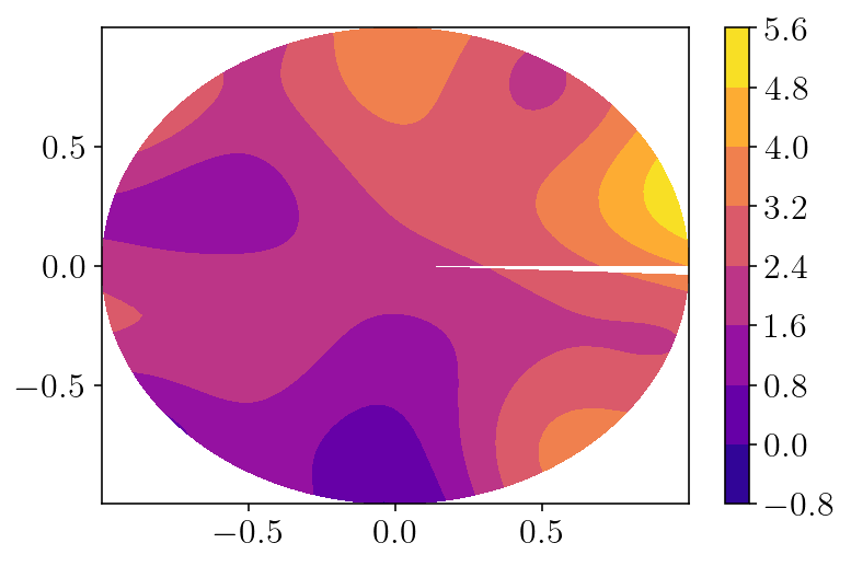
plotx = q2d_vol[:,0].reshape((nq_theta, nq_r))
plt.contourf(plotx, q2d_vol[:,1].reshape(plotx.shape), soln_fnc(q2d_vol[:,0], q2d_vol[:,1]).reshape(plotx.shape))
plt.colorbar()
plt.show()
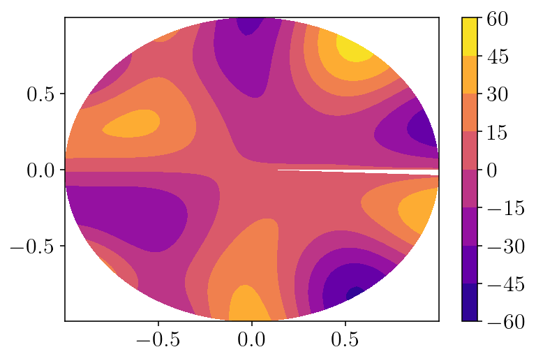
plotx = q2d_vol[:,0].reshape((nq_theta, nq_r))
plt.contourf(plotx, q2d_vol[:,1].reshape(plotx.shape), laplacian_fnc(q2d_vol[:,0], q2d_vol[:,1]).reshape(plotx.shape))
plt.colorbar()
plt.show()
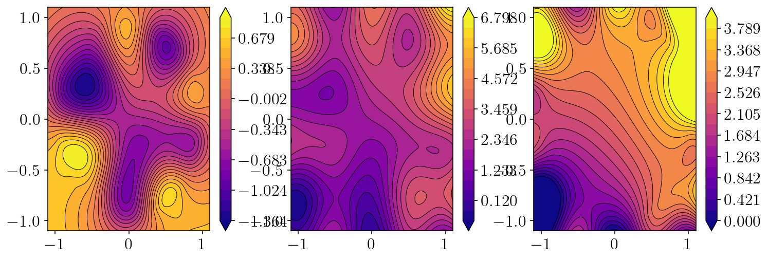
u_particular = (
    (single_layer.kernel(obs2d, q2d_vol, 0*q2d_vol)[:,0,:,0] * q2d_vol_wts[None,:])
    .dot(fxy)
    .reshape(obsx.shape)
)
plt.figure(figsize=(12,4))
plt.subplot(1,3,1)
levels = np.linspace(np.min(u_particular), np.max(u_particular), 21)
cntf = plt.contourf(obsx, obsy, u_particular, levels=levels, extend="both")
plt.contour(
    obsx,
    obsy,
    u_particular,
    colors="k",
    linestyles="-",
    linewidths=0.5,
    levels=levels,
    extend="both",
)
plt.colorbar(cntf)
plt.subplot(1,3,2)
levels = np.linspace(np.min(correct), np.max(correct), 21)
cntf = plt.contourf(obsx, obsy, correct, levels=levels, extend="both")
plt.contour(
    obsx,
    obsy,
    correct,
    colors="k",
    linestyles="-",
    linewidths=0.5,
    levels=levels,
    extend="both",
)
plt.colorbar(cntf)
plt.subplot(1,3,3)
err = correct - u_particular
levels = np.linspace(0, 4, 20)
cntf = plt.contourf(obsx, obsy, err, levels=levels, extend="both")
plt.contour(
    obsx,
    obsy,
    err,
    colors="k",
    linestyles="-",
    linewidths=0.5,
    levels=levels,
    extend="both",
)
plt.colorbar(cntf)
plt.show()
2.4. Direct to surface eval
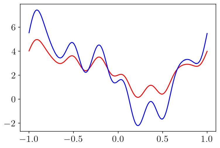
## This is g
bcs = soln_fnc(circle.pts[:, 0], circle.pts[:, 1])
## This is v|_{\partial \Omega}
surf_vals = (single_layer.kernel(circle.pts, q2d_vol)[:,0,:,0] * q2d_vol_wts[None,:]).dot(fxy)
A,report = integrate_term(double_layer, circle.pts, circle, return_report=True)
surf_density = np.linalg.solve(-A[:,0,:,0], bcs-surf_vals)
plt.plot(circle.quad_pts, bcs-surf_vals, 'r-')
plt.plot(circle.quad_pts, surf_density, 'b-')
plt.show()
%%time
interior_disp_mat = integrate_term(double_layer, obs2d, circle, tol=1e-13)
u_homog = -interior_disp_mat[:, 0, :, 0].dot(surf_density).reshape(obsx.shape)
CPU times: user 1.06 s, sys: 256 ms, total: 1.31 s
Wall time: 449 ms
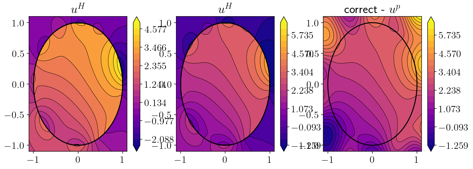
plt.figure(figsize=(12,4))
for i, to_plot in enumerate([u_homog, u_homog, correct - u_particular]):
plt.subplot(1,3,1+i)
if i == 0:
levels = np.linspace(np.min(to_plot), np.max(to_plot), 21)
else:
levels = np.linspace(np.min(correct - u_particular), np.max(correct - u_particular), 21)
cntf = plt.contourf(obsx, obsy, to_plot, levels=levels, extend="both")
plt.contour(
obsx,
obsy,
to_plot,
colors="k",
linestyles="-",
linewidths=0.5,
levels=levels,
extend="both",
)
plt.plot(circle.pts[:, 0], circle.pts[:, 1], "k-", linewidth=1.5)
plt.colorbar(cntf)
plt.xlim(zoomx)
plt.ylim(zoomy)
plt.title(['$u^H$', '$u^H$', 'correct - $u^p$'][i])
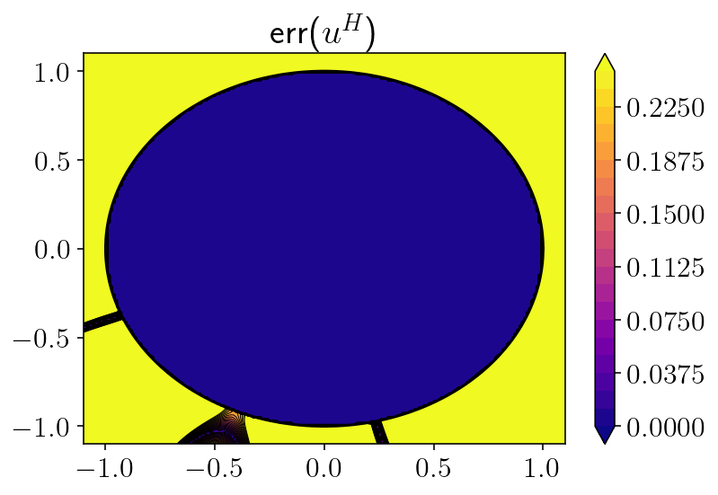
plt.figure()
to_plot = np.abs(correct - u_particular - u_homog)
levels = np.linspace(0, 0.25, 21)
cntf = plt.contourf(obsx, obsy, to_plot, levels=levels, extend="both")
plt.contour(
obsx,
obsy,
to_plot,
colors="k",
linestyles="-",
linewidths=0.5,
levels=levels,
extend="both",
)
plt.plot(circle.pts[:, 0], circle.pts[:, 1], "k-", linewidth=1.5)
plt.colorbar(cntf)
plt.xlim(zoomx)
plt.ylim(zoomy)
plt.title('err($u^H$)')
plt.show()
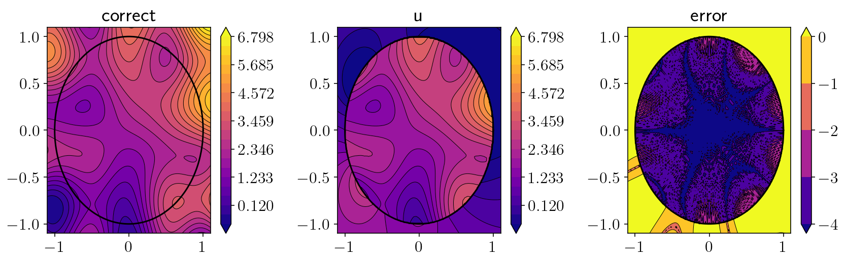
2.5. Full solution!
#u_full = u_box + u_particular
u_full = u_homog + u_particular
plt.figure(figsize=(12,4))
for i, to_plot in enumerate([correct, u_full]):
    plt.subplot(1,3,1+i)
    levels = np.linspace(np.min(correct), np.max(correct), 21)
    cntf = plt.contourf(obsx, obsy, to_plot, levels=levels, extend="both")
    plt.contour(
        obsx,
        obsy,
        to_plot,
        colors="k",
        linestyles="-",
        linewidths=0.5,
        levels=levels,
        extend="both",
    )
    plt.plot(circle.pts[:, 0], circle.pts[:, 1], "k-", linewidth=1.5)
    plt.colorbar(cntf)
    plt.xlim(zoomx)
    plt.ylim(zoomy)
    plt.title(['correct', 'u'][i])

plt.subplot(1,3,3)
to_plot = np.log10(np.abs(correct - u_full))
levels = np.linspace(-4, 0, 5)
cntf = plt.contourf(obsx, obsy, to_plot, levels=levels, extend="both")
plt.contour(
    obsx,
    obsy,
    to_plot,
    colors="k",
    linestyles="-",
    linewidths=0.5,
    levels=levels,
    extend="both",
)
plt.plot(circle.pts[:, 0], circle.pts[:, 1], "k-", linewidth=1.5)
plt.colorbar(cntf)
plt.xlim(zoomx)
plt.ylim(zoomy)
plt.title('error')
plt.tight_layout()
plt.show()
for norm in [np.linalg.norm, lambda x: np.linalg.norm(x, ord=1), lambda x: np.linalg.norm(x, ord=np.inf)]:
    A = norm(correct[obs2d_mask_sq] - u_full[obs2d_mask_sq])
    B = norm(correct[obs2d_mask_sq])
    print(A, B, A/B)
0.12040817419956851 387.36567421386707 0.00031083852342861536
11.0806270366859 57753.86762570072 0.00019185948045070793
0.008132634370805913 5.342989553063169 0.0015221130960556388
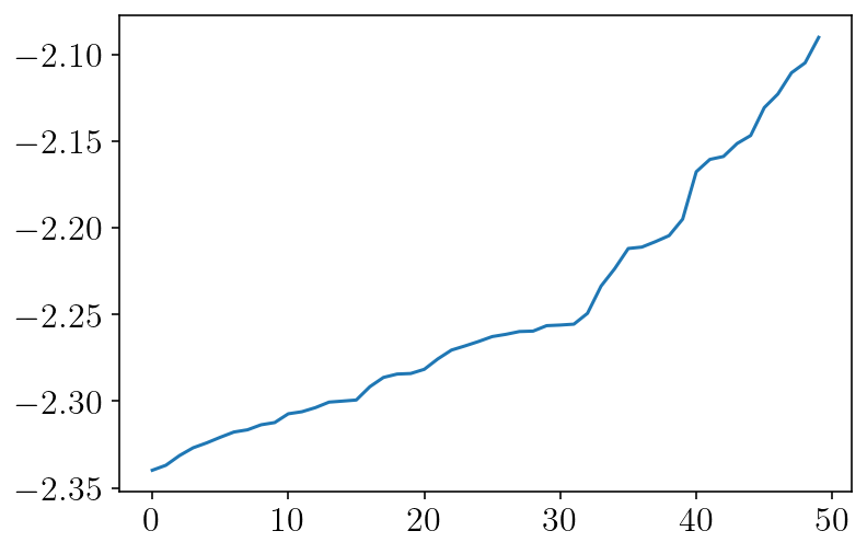
E = correct[obs2d_mask_sq] - u_full[obs2d_mask_sq]
plt.plot(np.log10(sorted(np.abs(E).tolist()))[-50:])
plt.show()