A fault and topography mesh of the South America subduction zone.
Contents
2. A fault and topography mesh of the South America subduction zone.
In the TDEs + Topography post, I used a mesh of the South America subduction zone. In this post, I thought it’d be fun to explain how I built that mesh.
import numpy as np
import scipy.io
import matplotlib.pyplot as plt

%config InlineBackend.figure_format='retina'
2.1. Looking at the fault model.
First off, I’m not going to explain how to build the fault geometry. That’s already been built! I’m using the same triangular subduction zone mesh used by Shannon Graham in her Global Block model papers. That mesh was built using the Slab 1.0 subduction zone contours. Also, the link in the Slab 1.0 paper is dead and the first Google search for Slab 1.0 is a portable cutting board.
Anyway… I’ll load the mesh up from the .mat file (a Matlab file format) and plot it.
file = scipy.io.loadmat("south_america_50km_mod_ext.mat")
fault_pts = file["c"]
fault_pts[:, 0] -= 360
fault_pts[:, 2] *= 1000
fault_tris = file["v"] - 1
I’m also going to plot the sign of vertical component of the normal vector just to check that all the triangles in the mesh are aligned in the same direction.
from cutde.geometry import compute_normal_vectors

normals = compute_normal_vectors(fault_pts[fault_tris])
plt.figure(figsize=(7, 8))
plt.subplot(1, 2, 1)
tripc = plt.tripcolor(
    fault_pts[:, 0],
    fault_pts[:, 1],
    fault_tris,
    fault_pts[:, 2] / 1000.0,
    linewidth=0.5,
)
plt.triplot(fault_pts[:, 0], fault_pts[:, 1], fault_tris, linewidth=0.5)
cbar = plt.colorbar()
cbar.set_label("depth (km)")
plt.xlim([np.min(fault_pts[:, 0]), np.max(fault_pts[:, 0])])
plt.axis("equal")
plt.xlabel("longitude")
plt.ylabel("latitude")
plt.subplot(1, 2, 2)
plt.tripcolor(fault_pts[:, 0], fault_pts[:, 1], fault_tris, np.sign(normals[:, 2]))
plt.colorbar()
plt.xlim([np.min(fault_pts[:, 0]), np.max(fault_pts[:, 0])])
plt.axis("equal")
plt.tight_layout()
plt.show()
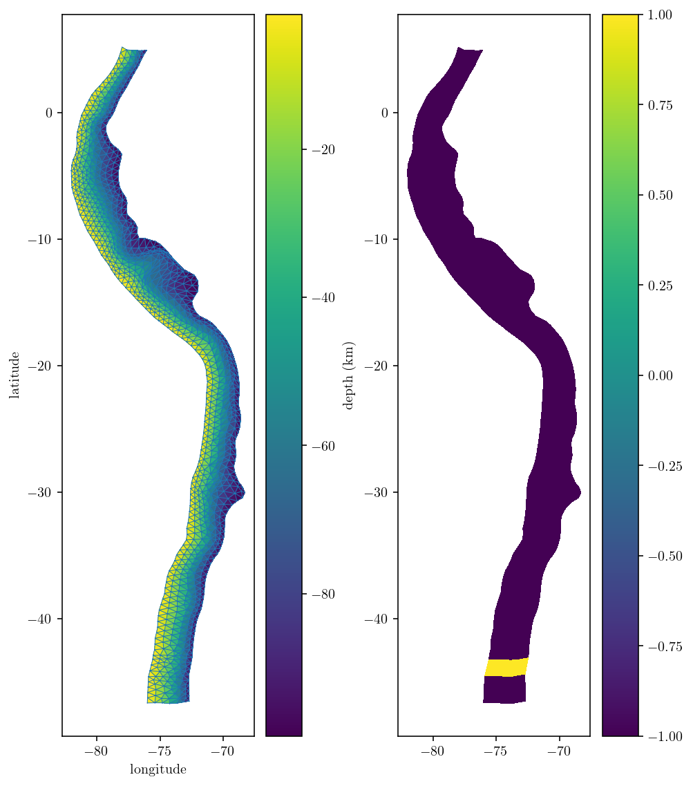
The mesh itself looks great at first glance! But, there is a mild problem with the element orientations at the southern end of the fault mesh. They don’t match the rest of the mesh. To fix the issue I can flip the triangle vertex ordering. Instead of ordering the vertices of a given triangle 0-1-2, I can flip the normal vector by ordering them 0-2-1. I’m actually going to flip the orientation of all the dark blue parts of the mesh since it’s a bit nicer to follow the convention that dipping fault normal vector point upwards. This convention results in an upwards-pointing dip vector which is consistent with the upwards dip-vector found in Okada.
flip_indices = np.where(normals[:, 2] < 0)
flag = np.zeros_like(normals[:, 0])
flag[flip_indices] = 1

flipped_tris = fault_tris.copy()
flipped_tris[flip_indices, 1] = fault_tris[flip_indices, 2]
flipped_tris[flip_indices, 2] = fault_tris[flip_indices, 1]
fault_tris = flipped_tris
2.2. Refining the fault mesh
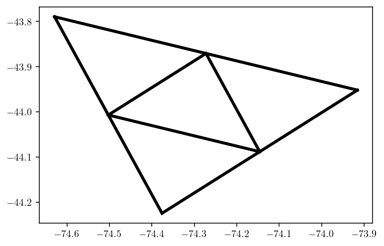
Depending on the situation, it might be nice to refine the fault mesh for more accuracy. A simple approach is to split each triangle into four new triangles based on the midpoints of each edge.
v0 = fault_pts[fault_tris[:, 0]]
v1 = fault_pts[fault_tris[:, 1]]
v2 = fault_pts[fault_tris[:, 2]]
v01 = 0.5 * (v0 + v1)
v02 = 0.5 * (v0 + v2)
v12 = 0.5 * (v1 + v2)
def plot_edge(a, b):
    P = np.array([a[0], b[0]])
    plt.plot(P[:, 0], P[:, 1], "k-")


plot_edge(v0, v1)
plot_edge(v2, v1)
plot_edge(v2, v0)
plot_edge(v01, v12)
plot_edge(v01, v02)
plot_edge(v12, v02)
new_pts = np.concatenate([fault_pts, v01, v02, v12])
v01_idxs = fault_pts.shape[0] + 0 * v01.shape[0] + np.arange(v01.shape[0])
v02_idxs = v01_idxs + v01.shape[0]
v12_idxs = v01_idxs + 2 * v01.shape[0]
import mesh_fncs

new_tris = np.array(
    [
        [fault_tris[:, 0], v01_idxs, v02_idxs],
        [fault_tris[:, 1], v12_idxs, v01_idxs],
        [fault_tris[:, 2], v02_idxs, v12_idxs],
        [v01_idxs, v12_idxs, v02_idxs],
    ]
)
new_tris = np.transpose(new_tris, (2, 0, 1)).reshape((-1, 3))
# fault_pts, fault_tris = mesh_fncs.remove_duplicate_pts((new_pts, new_tris))
2.3. Downloading DEM data
Now, let’s add surface topography and Earth curvature to this geometry. Why? Because, we can! And because we’re interested in the influence of realistic geometry. Also, I’ll end up projecting to geocentric coordinates where (X, Y, Z) = (0, 0, 0) is the center of the Earth.
Let’s start by Long ago I was using Mapzen for easily downloading DEM data. But Mapzen has gone out of business. So, I was sad and forlorn and had no easy source of DEM data… Until I discovered that Mapzen had exported their entire terrain tiles dataset to Amazon S3!. So, I replaced the old Mapzen API with some calls to AWS S3 using boto3. The basic API call is
def download_file(x, y, z, save_path):
    BUCKET_NAME = 'elevation-tiles-prod'
    KEY = 'geotiff/{z}/{x}/{y}.tif'.format(x = x, y = y, z = z)

    s3 = boto3.resource('s3')

    try:
        bucket = s3.Bucket(BUCKET_NAME)
        bucket.download_file(KEY, save_path)
    except botocore.exceptions.ClientError as e:
        if e.response['Error']['Code'] == "404":
            print("The object does not exist.")
        else:
            raise
I’ve wrapped this in a more advanced set of functions that allow passing a longitude-latitude bounding box and downloading the necessary files to create an interpolated digital elevation map.
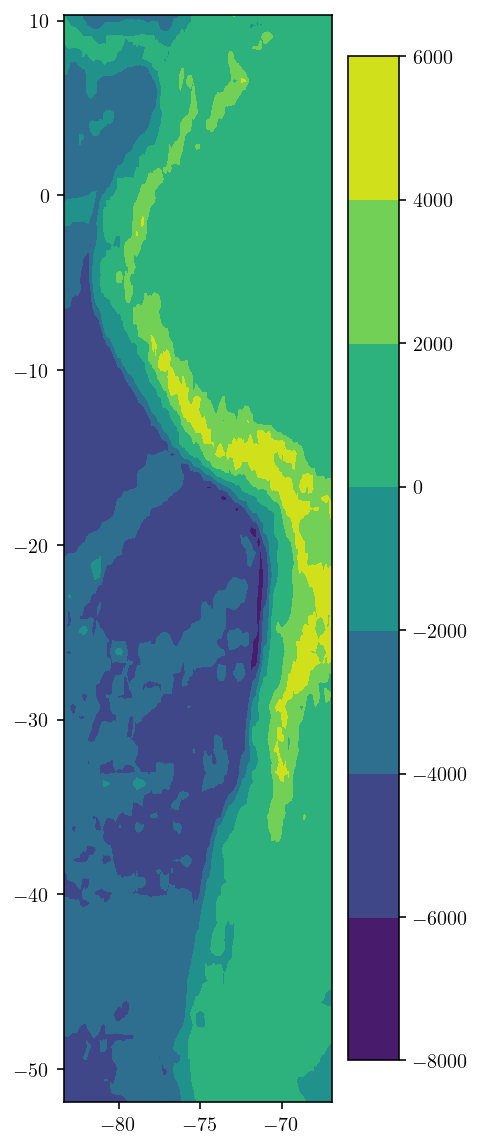
Let’s load up the module that does the DEM collection and just test out the tools. There are two relevant parameters: zoom determines the resolution of the DEM data. I’m grabbing a pretty large area of data, so I use a low zoom level of 2. And n_dem_interp_pts determines how many interpolation points are used to interpolate the DEM to our exact desired locations from the nearby provided coordinates.
import collect_dem

n_dem_interp_pts = 100
zoom = 2

bounds = collect_dem.get_dem_bounds(fault_pts)
dem_lon, dem_lat, dem = collect_dem.get_dem(zoom, bounds, n_dem_interp_pts)

plt.figure(figsize=(3, 10))
plt.tricontourf(dem_lon, dem_lat, dem)
plt.colorbar()
plt.show()
downloading dem data for bounds = [-51.875283536, -83.3826, 10.333847175999999, -66.93539999999999] and zoom = 2
10.333847175999999 -83.3826
-51.875283536 -66.93539999999999
Downloading /tmp/collected-fp0f_hlk/2-1-1.tif
Downloading /tmp/collected-fp0f_hlk/2-1-2.tif
Combining 2 into dem_download/raw_merc.tif ...
2.4. Building the surface mesh.
The next step is to build the surface mesh. However, not just any surface mesh. I need a surface mesh that “conforms” to the fault trace. To be precise, any fault mesh edge that intersects the surface should also be an edge in the surface mesh.
To do this, I’ll first identify the outer edges of the fault. This mesh_fncs module has a few handy functions for working with fault meshes like the get_boundary_loop function which returns the external edges of a surface mesh.
import mesh_fncs

boundary_loop = mesh_fncs.get_boundary_loop((fault_pts, fault_tris))[0]
plt.figure(figsize=(3, 10))
plt.plot(fault_pts[boundary_loop, 0], fault_pts[boundary_loop, 1], "-.")
plt.axis("equal")
plt.show()
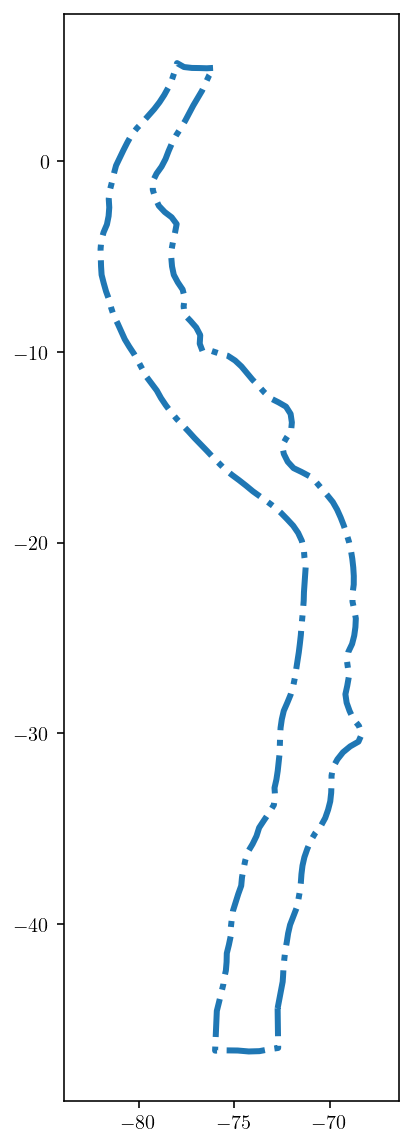
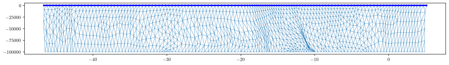
And then, just via trial and error, I found that boundary loop indices 130-258 correspond to the surface edges. This is demonstrated just by plotting those edges in the figure below where we looking from the side at the fault.
plt.figure(figsize=(16, 2.0))
upper_edge_idxs = boundary_loop[130:258]
# If we had refined the mesh above, this line will provide the
# correct upper_edge_idxs
# upper_edge_idxs = boundary_loop[259:514]
upper_edge_pts = fault_pts[upper_edge_idxs, :]
upper_edge_pts.shape
plt.plot(
    fault_pts[upper_edge_idxs, 1], fault_pts[upper_edge_idxs, 2], "b-*", markersize=4
)
plt.triplot(fault_pts[:, 1], fault_pts[:, 2], fault_tris, linewidth=0.5)
plt.show()
Next, we’re going to use pygmsh to interface with Gmsh and build our mesh. I’ll put some inline comments to explain what’s going on.
Note: I’m using pygmsh version 6.1.1 here.
import pygmsh

geom = pygmsh.built_in.Geometry()

# First, I'll figure out the area that I want to produce a surface mesh for.
# The center of the area will be the center of the fault.
surf_center = np.mean(upper_edge_pts, axis=0)
# And I also want to know the furthest that any fault mesh point is from that center point.
# This is essentially the fault "half-length"
fault_L = np.max(np.sqrt(np.sum((upper_edge_pts - surf_center) ** 2, axis=1)))
# The "half-width" of the surface mesh will be 1.5 times the fault half-length
w = fault_L * 1.5

# And the typical element length-scale will about one tenth the fault length.
# This length scale will only be relevant far from the fault. Near the fault,
# the length of the fault edges will force surface elements to be much smaller.
mesh_size_divisor = 4
mesh_size = fault_L / mesh_size_divisor

# The main polygon of the mesh is a big square.
surf_corners = np.array(
    [
        [surf_center[0] - w, surf_center[1] - w, 0],
        [surf_center[0] + w, surf_center[1] - w, 0],
        [surf_center[0] + w, surf_center[1] + w, 0],
        [surf_center[0] - w, surf_center[1] + w, 0],
    ]
)
surf = geom.add_polygon(surf_corners, mesh_size)

# Now, I'll add the fault trace edge points.
gmsh_pts = dict()
for i in range(upper_edge_pts.shape[0]):
    gmsh_pts[i] = geom.add_point(upper_edge_pts[i], mesh_size)

# And this chunk of code specifies that those edges should be
# included in the surface mesh.
for i in range(1, upper_edge_pts.shape[0]):
    line = geom.add_line(gmsh_pts[i - 1], gmsh_pts[i])

    # pygmsh didn't support this elegantly, so I just insert manual gmsh code.
    intersection_code = "Line{{{}}} In Surface{{{}}};".format(line.id, surf.surface.id)
    geom.add_raw_code(intersection_code)
Finally, build the geometry and can generate the surface mesh.
mesh = pygmsh.generate_mesh(geom, dim=2)
Info    : Running 'gmsh -2 /tmp/tmp2_wpi6tj.geo -format msh -bin -o /tmp/tmpsxv71cza.msh' [Gmsh 4.6.0, 1 node, max. 1 thread]
Info    : Started on Mon Apr 26 20:35:25 2021
Info    : Reading '/tmp/tmp2_wpi6tj.geo'...
Info    : Done reading '/tmp/tmp2_wpi6tj.geo'
Info    : Meshing 1D...
Info    : [  0%] Meshing curve 1 (Line)
Info    : [ 10%] Meshing curve 2 (Line)
Info    : [ 10%] Meshing curve 3 (Line)
Info    : [ 10%] Meshing curve 4 (Line)
Info    : [ 10%] Meshing curve 7 (Line)
Info    : [ 10%] Meshing curve 8 (Line)
Info    : [ 10%] Meshing curve 9 (Line)
Info    : [ 10%] Meshing curve 10 (Line)
Info    : [ 10%] Meshing curve 11 (Line)
Info    : [ 10%] Meshing curve 12 (Line)
Info    : [ 10%] Meshing curve 13 (Line)
Info    : [ 10%] Meshing curve 14 (Line)
Info    : [ 10%] Meshing curve 15 (Line)
Info    : [ 10%] Meshing curve 16 (Line)
Info    : [ 20%] Meshing curve 17 (Line)
Info    : [ 20%] Meshing curve 18 (Line)
Info    : [ 20%] Meshing curve 19 (Line)
Info    : [ 20%] Meshing curve 20 (Line)
Info    : [ 20%] Meshing curve 21 (Line)
Info    : [ 20%] Meshing curve 22 (Line)
Info    : [ 20%] Meshing curve 23 (Line)
Info    : [ 20%] Meshing curve 24 (Line)
Info    : [ 20%] Meshing curve 25 (Line)
Info    : [ 20%] Meshing curve 26 (Line)
Info    : [ 20%] Meshing curve 27 (Line)
Info    : [ 20%] Meshing curve 28 (Line)
Info    : [ 20%] Meshing curve 29 (Line)
Info    : [ 30%] Meshing curve 30 (Line)
Info    : [ 30%] Meshing curve 31 (Line)
Info    : [ 30%] Meshing curve 32 (Line)
Info    : [ 30%] Meshing curve 33 (Line)
Info    : [ 30%] Meshing curve 34 (Line)
Info    : [ 30%] Meshing curve 35 (Line)
Info    : [ 30%] Meshing curve 36 (Line)
Info    : [ 30%] Meshing curve 37 (Line)
Info    : [ 30%] Meshing curve 38 (Line)
Info    : [ 30%] Meshing curve 39 (Line)
Info    : [ 30%] Meshing curve 40 (Line)
Info    : [ 30%] Meshing curve 41 (Line)
Info    : [ 30%] Meshing curve 42 (Line)
Info    : [ 40%] Meshing curve 43 (Line)
Info    : [ 40%] Meshing curve 44 (Line)
Info    : [ 40%] Meshing curve 45 (Line)
Info    : [ 40%] Meshing curve 46 (Line)
Info    : [ 40%] Meshing curve 47 (Line)
Info    : [ 40%] Meshing curve 48 (Line)
Info    : [ 40%] Meshing curve 49 (Line)
Info    : [ 40%] Meshing curve 50 (Line)
Info    : [ 40%] Meshing curve 51 (Line)
Info    : [ 40%] Meshing curve 52 (Line)
Info    : [ 40%] Meshing curve 53 (Line)
Info    : [ 40%] Meshing curve 54 (Line)
Info    : [ 40%] Meshing curve 55 (Line)
Info    : [ 50%] Meshing curve 56 (Line)
Info    : [ 50%] Meshing curve 57 (Line)
Info    : [ 50%] Meshing curve 58 (Line)
Info    : [ 50%] Meshing curve 59 (Line)
Info    : [ 50%] Meshing curve 60 (Line)
Info    : [ 50%] Meshing curve 61 (Line)
Info    : [ 50%] Meshing curve 62 (Line)
Info    : [ 50%] Meshing curve 63 (Line)
Info    : [ 50%] Meshing curve 64 (Line)
Info    : [ 50%] Meshing curve 65 (Line)
Info    : [ 50%] Meshing curve 66 (Line)
Info    : [ 50%] Meshing curve 67 (Line)
Info    : [ 50%] Meshing curve 68 (Line)
Info    : [ 60%] Meshing curve 69 (Line)
Info    : [ 60%] Meshing curve 70 (Line)
Info    : [ 60%] Meshing curve 71 (Line)
Info    : [ 60%] Meshing curve 72 (Line)
Info    : [ 60%] Meshing curve 73 (Line)
Info    : [ 60%] Meshing curve 74 (Line)
Info    : [ 60%] Meshing curve 75 (Line)
Info    : [ 60%] Meshing curve 76 (Line)
Info    : [ 60%] Meshing curve 77 (Line)
Info    : [ 60%] Meshing curve 78 (Line)
Info    : [ 60%] Meshing curve 79 (Line)
Info    : [ 60%] Meshing curve 80 (Line)
Info    : [ 60%] Meshing curve 81 (Line)
Info    : [ 70%] Meshing curve 82 (Line)
Info    : [ 70%] Meshing curve 83 (Line)
Info    : [ 70%] Meshing curve 84 (Line)
Info    : [ 70%] Meshing curve 85 (Line)
Info    : [ 70%] Meshing curve 86 (Line)
Info    : [ 70%] Meshing curve 87 (Line)
Info    : [ 70%] Meshing curve 88 (Line)
Info    : [ 70%] Meshing curve 89 (Line)
Info    : [ 70%] Meshing curve 90 (Line)
Info    : [ 70%] Meshing curve 91 (Line)
Info    : [ 70%] Meshing curve 92 (Line)
Info    : [ 70%] Meshing curve 93 (Line)
Info    : [ 70%] Meshing curve 94 (Line)
Info    : [ 80%] Meshing curve 95 (Line)
Info    : [ 80%] Meshing curve 96 (Line)
Info    : [ 80%] Meshing curve 97 (Line)
Info    : [ 80%] Meshing curve 98 (Line)
Info    : [ 80%] Meshing curve 99 (Line)
Info    : [ 80%] Meshing curve 100 (Line)
Info    : [ 80%] Meshing curve 101 (Line)
Info    : [ 80%] Meshing curve 102 (Line)
Info    : [ 80%] Meshing curve 103 (Line)
Info    : [ 80%] Meshing curve 104 (Line)
Info    : [ 80%] Meshing curve 105 (Line)
Info    : [ 80%] Meshing curve 106 (Line)
Info    : [ 80%] Meshing curve 107 (Line)
Info    : [ 90%] Meshing curve 108 (Line)
Info    : [ 90%] Meshing curve 109 (Line)
Info    : [ 90%] Meshing curve 110 (Line)
Info    : [ 90%] Meshing curve 111 (Line)
Info    : [ 90%] Meshing curve 112 (Line)
Info    : [ 90%] Meshing curve 113 (Line)
Info    : [ 90%] Meshing curve 114 (Line)
Info    : [ 90%] Meshing curve 115 (Line)
Info    : [ 90%] Meshing curve 116 (Line)
Info    : [ 90%] Meshing curve 117 (Line)
Info    : [ 90%] Meshing curve 118 (Line)
Info    : [ 90%] Meshing curve 119 (Line)
Info    : [ 90%] Meshing curve 120 (Line)
Info    : [100%] Meshing curve 121 (Line)
Info    : [100%] Meshing curve 122 (Line)
Info    : [100%] Meshing curve 123 (Line)
Info    : [100%] Meshing curve 124 (Line)
Info    : [100%] Meshing curve 125 (Line)
Info    : [100%] Meshing curve 126 (Line)
Info    : [100%] Meshing curve 127 (Line)
Info    : [100%] Meshing curve 128 (Line)
Info    : [100%] Meshing curve 129 (Line)
Info    : [100%] Meshing curve 130 (Line)
Info    : [100%] Meshing curve 131 (Line)
Info    : [100%] Meshing curve 132 (Line)
Info    : [100%] Meshing curve 133 (Line)
Info    : Done meshing 1D (Wall 0.0103769s, CPU 0.03271s)
Info    : Meshing 2D...
Info    : Meshing surface 6 (Plane, Frontal-Delaunay)
Info    : Done meshing 2D (Wall 0.078131s, CPU 0.196172s)
Info    : 1931 nodes 4119 elements
Info    : Writing '/tmp/tmpsxv71cza.msh'...
Info    : Done writing '/tmp/tmpsxv71cza.msh'
Info    : Stopped on Mon Apr 26 20:35:25 2021 (From start: Wall 0.101154s, CPU 0.340551s)
Let’s plot the resulting mesh. The output format is from the meshio package.
surf_pts = mesh.points
surf_tris = mesh.cells_dict["triangle"]

plt.figure(figsize=(10, 10))
plt.triplot(surf_pts[:, 0], surf_pts[:, 1], surf_tris, linewidth=0.5)
plt.plot(
    upper_edge_pts[:, 0], upper_edge_pts[:, 1], "k-", linewidth=1.0
)  # , markersize = 2)
vW = 1.1 * w
plt.xlim([surf_center[0] - vW, surf_center[0] + vW])
plt.ylim([surf_center[1] - vW, surf_center[1] + vW])
plt.show()
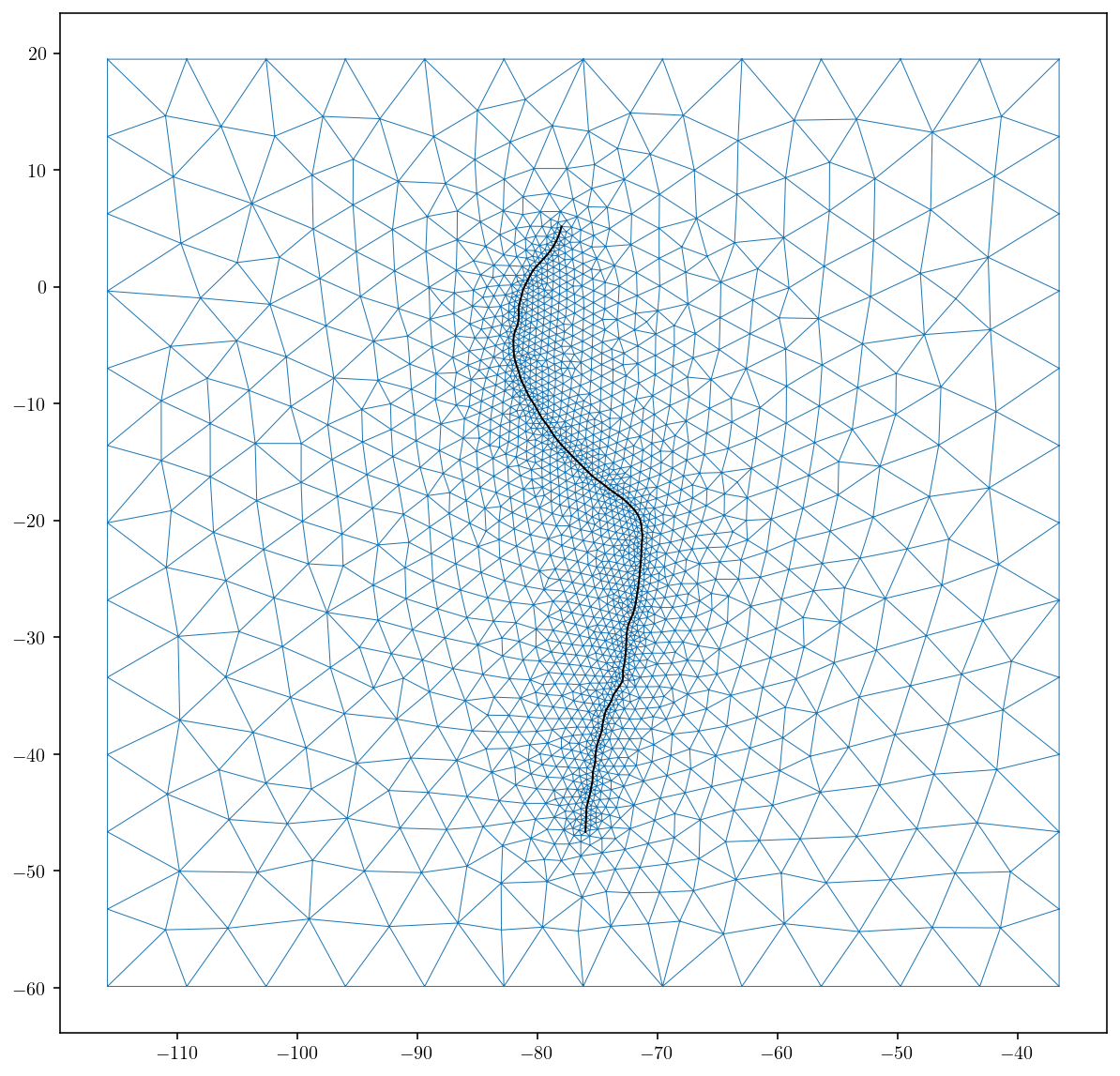
Great, that’s exactly what I was going for. A mesh that conforms to the fault trace and also gets smoothly coarser moving away from the fault trace.
The final step is to set elevation:
the elevation for the surface mesh. It’s currently zero everywhere.
I also offset the fault model based on the surface elevation since the Slab 1.0 models are defined in terms of depth below the surface.
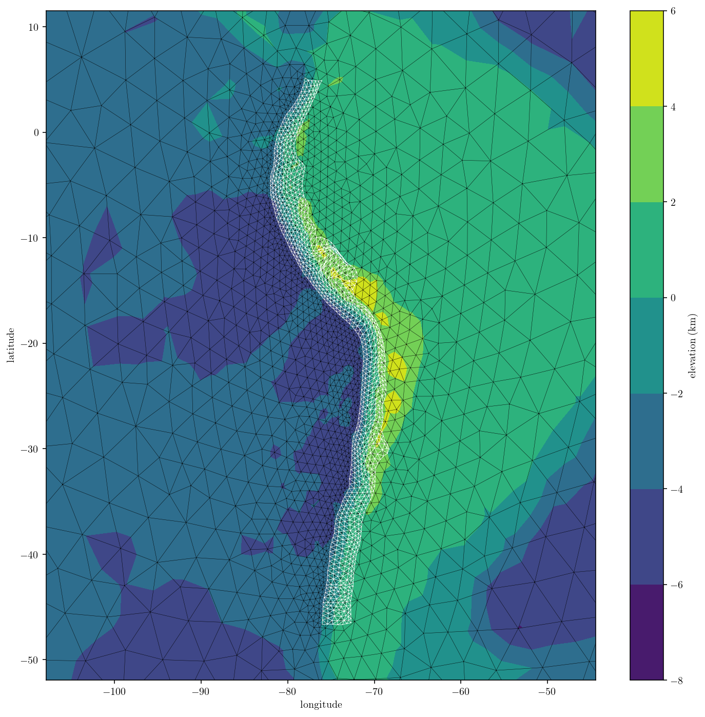
Note that because we use the same DEM data for computing surface and fault elevations, that the fault trace and the surface edges will precisely match. Using different DEM data for each mesh is a common error here that will result in gaps that may or may not matter depending on the end goal.
bounds = collect_dem.get_dem_bounds(surf_pts)
LON, LAT, DEM = collect_dem.get_dem(zoom, bounds, n_dem_interp_pts)

surf_pts[:, 2] = scipy.interpolate.griddata(
    (LON, LAT), DEM, (surf_pts[:, 0], surf_pts[:, 1])
)
fault_pts[:, 2] += scipy.interpolate.griddata(
    (LON, LAT), DEM, (fault_pts[:, 0], fault_pts[:, 1])
)
downloading dem data for bounds = [-67.80746557203787, -123.7930824435223, 27.407324315006626, -28.5782925564778] and zoom = 2
27.407324315006626 -123.7930824435223
-67.80746557203787 -28.5782925564778
Downloading /tmp/collected-ohginqx3/2-0-1.tif
Downloading /tmp/collected-ohginqx3/2-1-1.tif
Downloading /tmp/collected-ohginqx3/2-0-2.tif
Downloading /tmp/collected-ohginqx3/2-1-2.tif
Downloading /tmp/collected-ohginqx3/2-0-3.tif
Downloading /tmp/collected-ohginqx3/2-1-3.tif
Combining 6 into dem_download/raw_merc.tif ...
And I’ll make a simple plot of the final mesh. Looks good!
plt.figure(figsize=(12, 12))
cntf = plt.tricontourf(
    surf_pts[:, 0], surf_pts[:, 1], surf_tris, surf_pts[:, 2] / 1000.0
)
plt.triplot(surf_pts[:, 0], surf_pts[:, 1], surf_tris, "k-", linewidth=0.25)
plt.triplot(fault_pts[:, 0], fault_pts[:, 1], fault_tris, "w-", linewidth=0.4)
vW = 1.2 * fault_L
plt.xlim([surf_center[0] - vW, surf_center[0] + vW])
plt.ylim([surf_center[1] - vW, surf_center[1] + vW])
cbar = plt.colorbar()
cbar.set_label("elevation (km)")
plt.xlabel("longitude")
plt.ylabel("latitude")
plt.show()
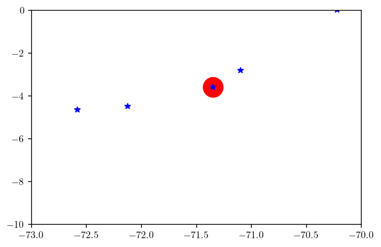
Let’s zoom in on an longitude-z plane approximate cross section of the fault and surface to check that the fault trace and surface match up. The big red dot is a fault mesh point while the blue stars show the points in the cross section from the surface mesh.
idxs = (fault_pts[:, 1] < -20) & (fault_pts[:, 1] > -20.5)
plt.plot(fault_pts[idxs, 0], fault_pts[idxs, 2] / 1000.0, "ro", markersize=20)
idxs = (surf_pts[:, 1] < -20) & (surf_pts[:, 1] > -20.5)
plt.plot(surf_pts[idxs, 0], surf_pts[idxs, 2] / 1000.0, "b*")
plt.xlim([-73, -70])
plt.ylim([-10, 0])
plt.show()
Awesome! The mesh is ready to use and I’ll save it to disk for safe-keeping.
np.save(
    f"sa_mesh{mesh_size_divisor}_{fault_tris.shape[0]}.npy",
    np.array([(surf_pts, surf_tris), (fault_pts, fault_tris)], dtype=object),
)