Minimizing memory usage: a matrix-free iterative solver
Contents
3. Minimizing memory usage: a matrix-free iterative solver
3.1. How to deal with dense BEM matrices?
In the previous section, I explained how to directly discretize a free surface using TDEs. A downside of this approach is that the surface matrix can get very large very quickly. If I make the width of an element half as large, then there will be 2x many elements per dimension and 4x as many elements overall. And because the interaction matrix is dense, 4x as many elements leads to 16x as many matrix entries. In other words, \(n\), the number of elements, scales like \(O(h^2)\) in terms of the element width \(h\). And the number of matrix rows or columns is exactly \(3n\) (the 3 comes from the vector nature of the problem). That requires storing \(9n^2\) entries. And, even worse, using a direct solver (LU decomposition, Gaussian elimination, etc) with such a matrix requires time like \(O(n^3)\). Even for quite small problems with 10,000 elements, the cost of storage and solution get very large. And without an absolutely enormous machine or a distributed parallel implementation, solving a problem with 200,000 elements will just not be possible. On the other hand, in an ideal world, it would be nice to be able to solve problems with millions or even tens or hundreds of millions of elements.
Fundamentally, the problem is that the interaction matrix is dense. There are two approaches for resolving this problem:
Don’t store the matrix!
Compress the matrix by taking advantage of low rank sub-blocks.
Eventually approach #2 will be critical since it is scalable up to very large problems. And that’s exactly what I’ll do in the next sections where I’ll investigate low-rank methods and hierarchical matrices (H-matrices). However, here, I’ll demonstrate approach #1 by using a matrix-free iterative solver. Ultimately, this is just a small patch on a big problem and it won’t be a sustainable solution. But, it’s immediately useful when you don’t have a working implementation, are running into RAM constraints and are okay with a fairly slow solution. It’s also useful to introduce iterative linear solvers since they are central to solving BEM linear systems.
When we solve a linear system without storing the matrix, the method is called “matrix-free”. Generally, we’ll just recompute any matrix entry whenever we need. How does this do algorithmically? The storage requirements drop to just the \(O(n)\) source and observation info instead of the \(O(n^2)\) dense matrix. And, as I’ll demonstrate, for some problems, the runtime will drop to \(O(n^2)\) instead of \(O(n^3)\) because solving linear systems will be possible with a fixed and fairly small number of matrix-vector products.
3.2. A demonstration on a large mesh.
To get started, I’ll just copy the code to set up the linear system for the South America problem from the previous section. But, as a twist, I’ll going to use a mesh with several times more elements. This surface mesh has 28,388 elements. As a result, the matrix would have 3x that many rows and columns and would require 58 GB of memory to store. That’s still small enough that it could be stored on a medium sized workstation. But, it’s too big for my personal computer!
import cutde.fullspace as FS
import cutde.geometry
import numpy as np
import matplotlib.pyplot as plt
from pyproj import Transformer

plt.rcParams["text.usetex"] = True
%config InlineBackend.figure_format='retina'
(surf_pts_lonlat, surf_tris), (fault_pts_lonlat, fault_tris) = np.load(
    "sa_mesh16_7216.npy", allow_pickle=True
)
print("Memory required to store this matrix: ", (surf_tris.shape[0] * 3) ** 2 * 8 / 1e9)
Memory required to store this matrix: 58.023255168
transformer = Transformer.from_crs(
    "+proj=longlat +ellps=WGS84 +datum=WGS84 +no_defs",
    "+proj=geocent +datum=WGS84 +units=m +no_defs",
)
surf_pts_xyz = np.array(
    transformer.transform(
        surf_pts_lonlat[:, 0], surf_pts_lonlat[:, 1], surf_pts_lonlat[:, 2]
    )
).T.copy()
fault_pts_xyz = np.array(
    transformer.transform(
        fault_pts_lonlat[:, 0], fault_pts_lonlat[:, 1], fault_pts_lonlat[:, 2]
    )
).T.copy()

surf_tri_pts_xyz = surf_pts_xyz[surf_tris]
surf_xyz_to_tdcs_R = cutde.geometry.compute_efcs_to_tdcs_rotations(surf_tri_pts_xyz)

fault_centers_lonlat = np.mean(fault_pts_lonlat[fault_tris], axis=1)
fault_lonlat_to_xyz_T = cutde.geometry.compute_projection_transforms(
    fault_centers_lonlat, transformer
)

fault_tri_pts_xyz = fault_pts_xyz[fault_tris]
# Compute the transformation from spherical xyz coordinates (the "EFCS" - Earth fixed coordinate system)
fault_xyz_to_tdcs_R = cutde.geometry.compute_efcs_to_tdcs_rotations(fault_tri_pts_xyz)

fault_tri_pts_lonlat = fault_pts_lonlat[fault_tris]
fault_tdcs2_to_lonlat_R = cutde.geometry.compute_efcs_to_tdcs_rotations(fault_tri_pts_lonlat)

strike_lonlat = fault_tdcs2_to_lonlat_R[:, 0, :]
dip_lonlat = fault_tdcs2_to_lonlat_R[:, 1, :]

strike_xyz = np.sum(fault_lonlat_to_xyz_T * strike_lonlat[:, None, :], axis=2)
strike_xyz /= np.linalg.norm(strike_xyz, axis=1)[:, None]
dip_xyz = np.sum(fault_lonlat_to_xyz_T * dip_lonlat[:, None, :], axis=2)
dip_xyz /= np.linalg.norm(dip_xyz, axis=1)[:, None]

# The normal vectors for each triangle are the third rows of the XYZ->TDCS rotation matrices.
Vnormal = surf_xyz_to_tdcs_R[:, 2, :]
surf_centers_xyz = np.mean(surf_tri_pts_xyz, axis=1)
surf_tri_pts_xyz_conv = surf_tri_pts_xyz.astype(np.float32)

# The rotation matrix from TDCS to XYZ is the transpose of XYZ to TDCS.
# The inverse of a rotation matrix is its transpose.
surf_tdcs_to_xyz_R = np.transpose(surf_xyz_to_tdcs_R, (0, 2, 1)).astype(np.float32)
Proceeding like the previous section, the next step would be to construct our surface to surface left hand side matrix. But, instead, I’m just going to compute the action of that matrix without ever storing the entire matrix. Essentially, each matrix entry will be recomputed whenever it is needed. The cutde.disp_free and cutde.strain_free were written for this purpose.
First, let’s check that the cutde.disp_free matrix free TDE computation is doing what I said it does. That is, it should be computing a matrix vector product. Since our problem is too big to generate the full matrix in memory, I’ll just use the first 100 elements for this test.
First, I’ll compute the full in-memory matrix subset. This should look familiar! Then, I multiply the matrix by a random slip vector.
test_centers = (surf_centers_xyz - 1.0 * Vnormal)[:100].astype(np.float32)
mat = FS.disp_matrix(test_centers, surf_tri_pts_xyz_conv[:100], 0.25).reshape(
    (300, 300)
)
slip = np.random.rand(mat.shape[1]).astype(np.float32)
correct_disp = mat.dot(slip)
And now the matrix free version. Note that the slip is passed to the disp_free function. This makes sense since it is required for a matrix-vector product even though it is not required to construct the matrix with cutde.disp_matrix.
test_disp = FS.disp_free(
    test_centers, surf_tri_pts_xyz_conv[:100], slip.reshape((-1, 3)), 0.25
)
And let’s calculate the error… It looks good for the first element. For 32-bit floats, this is machine precision.
err = correct_disp.reshape((-1, 3)) - test_disp
err[0]
array([ 6.5565109e-07, -4.7683716e-07, -2.1606684e-07], dtype=float32)
np.mean(np.abs(err)), np.max(np.abs(err))
(2.8643137e-07, 1.0877848e-06)
Okay, now that I’ve shown that cutde.disp_free is trustworthy, let’s construct a function that computes matrix vector products of the (not in memory) left-hand side matrix.
To start, recall the linear system that we are solving from the last section:
where \(H_i\) is a free surface TDE, \(\overline{H_i}\) is the centroid of that TDE, \(F_j\) is a fault TDE, \(\Delta u_j\) is the imposed slip field and \(x=u_j\) is the unknown surface displacement field.
Implicitly, in the construction of that left hand side matrix, there are a number of rotations embedded in the TDE operations. There’s also an extrapolation step that we introduced in the last section that allows for safely evaluated at observation points that are directly on the source TDE. We need to transform all those rotation and extrapolation steps into a form that makes sense in an “on the fly” setting where we’re not storing a matrix. The matvec function does exactly this.
offsets = [2.0, 1.0]
offset_centers = [(surf_centers_xyz - off * Vnormal).astype(np.float32) for off in offsets]

# The matrix that will rotate from (x, y, z) into
# the TDCS (triangular dislocation coordinate system)
surf_xyz_to_tdcs_R = surf_xyz_to_tdcs_R.astype(np.float32)

# The extrapolate to the boundary step looked like:
# lhs = 2 * eps_mats[1] - eps_mats[0]
# This array stores the coefficients so that we can apply that formula
# on the fly.
extrapolation_mult = [-1, 2]


def matvec(disp_xyz_flattened):
    # Step 0) Unflatten the (x,y,z) coordinate displacement vector.
    disp_xyz = disp_xyz_flattened.reshape((-1, 3)).astype(ft)

    # Step 1) Rotate displacement into the TDCS (triangular dislocation coordinate system).
    disp_tdcs = np.ascontiguousarray(
        np.sum(surf_xyz_to_tdcs_R * disp_xyz[:, None, :], axis=2)
    )

    # Step 2) Compute the two point extrapolation to the boundary.
    # Recall from the previous section that this two point extrapolation
    # allow us to calculate for observation points that lie right on a TDE
    # without worrying about numerical inaccuracies.
    out = np.zeros_like(offset_centers[0])
    for i in range(len(offsets)):
        out += extrapolation_mult[i] * FS.disp_free(
            offset_centers[i], surf_tri_pts_xyz_conv, disp_tdcs, 0.25
        )
    out = out.flatten()

    # Step 3) Don't forget the diagonal Identity matrix term!
    out += disp_xyz_flattened
    return out
%%time
matvec(np.random.rand(surf_tris.shape[0] * 3))
CPU times: user 5min 27s, sys: 7.21 s, total: 5min 34s
Wall time: 55.4 s
array([-0.15508433,  0.21774934,  0.0313065 , ...,  0.02519985,
        0.26969355, -0.00616684], dtype=float32)
Great! We computed a matrix-free matrix-vector product! Unfortunately, it’s a bit slow, but that’s an unsurprising consequence of running an \(O(n^2)\) algorithm for a large value of \(n\). The nice thing is that we’re able to do this at all by not storing the matrix at any point. This little snippet below will demonstrate that the memory usage is still well under 1 GB proving that we’re not storing a matrix anywhere.
import os, psutil

process = psutil.Process(os.getpid())
print(process.memory_info().rss / 1e9)
0.146767872
3.3. Iterative linear solution
Okay, so how do we use this matrix-vector product to solve the linear system? Because the entire matrix is never in memory, direct solvers like LU decomposition or Cholesky decomposition are no longer an option. But, iterative linear solvers are still an option. The conjugate gradient (CG) method is a well-known example of an iterative solver. However, CG requires a symmetric positive definite matrix. Because our columns come from integrals over elements but our rows come from observation points, there is an inherent asymmetry to the boundary element matrices we are producing here. GMRES is an iterative linear solver that tolerates asymmetry. It’s specifically a type of “Krylov subspace” iterative linear solver and as such requires only the set of vectors:
As such, only having an implementation of the matrix vector product \(Ab\) is required since the later iterates can be computed with multiple matrix vector product. For example, \(A^2b = A(Ab)\).
Returning to our linear system above, the right hand side is the amount of displacement at the free surface caused by slip on the fault and can be precomputed because it is only a vector (and thus doesn’t require much memory) and will not change during our linear solve.
slip = np.ascontiguousarray(np.sum(fault_xyz_to_tdcs_R * dip_xyz[:, None, :], axis=2), dtype=np.float32)
rhs = FS.disp_free(
    surf_centers_xyz.astype(np.float32), fault_pts_xyz[fault_tris].astype(np.float32), slip, 0.25
).flatten()
Now, the fun stuff: Here, I’ll use the scipy implementation of GMRES. First, we need to do use the scipy.sparse.linalg.LinearOperator interface to wrap our matvec function in a form that the gmres function will recognize as a something that represents a linear system that can be solved.
import time
import scipy.sparse.linalg as spla

# The number of rows and columns
n = surf_tris.shape[0] * 3

# The matrix vector product function that serves as the "backend" for the LinearOperator.
# This is just a handy wrapper around matvec to track the number of matrix-vector products
# used during the linear solve process.
def M(disp_xyz_flattened):
    M.n_iter += 1
    start = time.time()
    out = matvec(disp_xyz_flattened)
    print("n_matvec", M.n_iter, "took", time.time() - start)
    return out


M.n_iter = 0
lhs = spla.LinearOperator((n, n), M, dtype=rhs.dtype)
lhs.shape
(85164, 85164)
And then we can pass that LinearOperator as the left hand side of a system of equations to gmres. I’m also going to pass a simple callback that will print the current residual norm at each step of the iterative solver and require a solution tolerance of 1e-4.
np.linalg.norm(rhs)
26.986288
soln = spla.gmres(
    lhs,
    rhs,
    tol=1e-4,
    atol=1e-4,
    restart=100,
    maxiter=1,
    callback_type="pr_norm",
    callback=lambda x: print(x),
)
soln = soln[0].reshape((-1, 3))
n_matvec 1 took 8.181740522384644
n_matvec 2 took 8.217356204986572
0.21284150158882
n_matvec 3 took 8.110730171203613
0.026337904611568017
n_matvec 4 took 8.143013715744019
0.0058701005433943266
n_matvec 5 took 8.101205348968506
0.0016042871687649372
n_matvec 6 took 8.221377849578857
0.0004220627227557851
n_matvec 7 took 8.234569311141968
9.5677343550821e-05
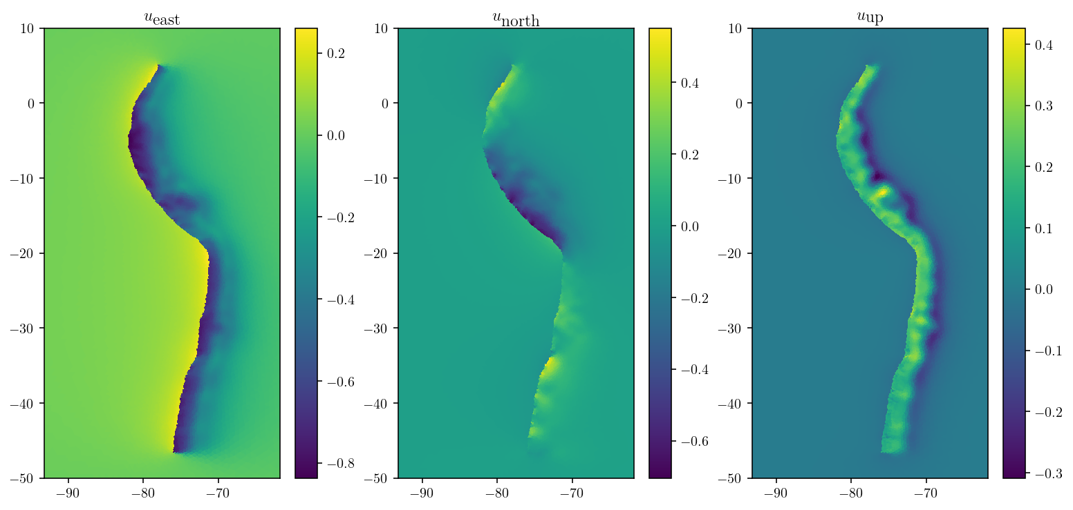
As the figures below demonstrate, only eight matrix-vector products got us a great solution!
inverse_transformer = Transformer.from_crs(
    "+proj=geocent +datum=WGS84 +units=m +no_defs",
    "+proj=longlat +ellps=WGS84 +datum=WGS84 +no_defs",
)
surf_xyz_to_lonlat_T = cutde.compute_projection_transforms(
    surf_centers_xyz, inverse_transformer
)
surf_xyz_to_lonlat_T /= np.linalg.norm(surf_xyz_to_lonlat_T, axis=2)[:, :, None]
soln_lonlat = np.sum(surf_xyz_to_lonlat_T * soln[:, None, :], axis=2)

plt.figure(figsize=(13, 6))
for d in range(3):
    plt.subplot(1, 3, 1 + d)
    cntf = plt.tripcolor(
        surf_pts_lonlat[:, 0], surf_pts_lonlat[:, 1], surf_tris, soln_lonlat[:, d]
    )
    plt.colorbar(cntf)
    plt.axis("equal")
    plt.xlim([-85, -70])
    plt.ylim([-50, 10])
    plt.title(
        ["$u_{\\textrm{east}}$", "$u_{\\textrm{north}}$", "$u_{\\textrm{up}}$"][d]
    )
plt.show()
3.4. Performance and convergence
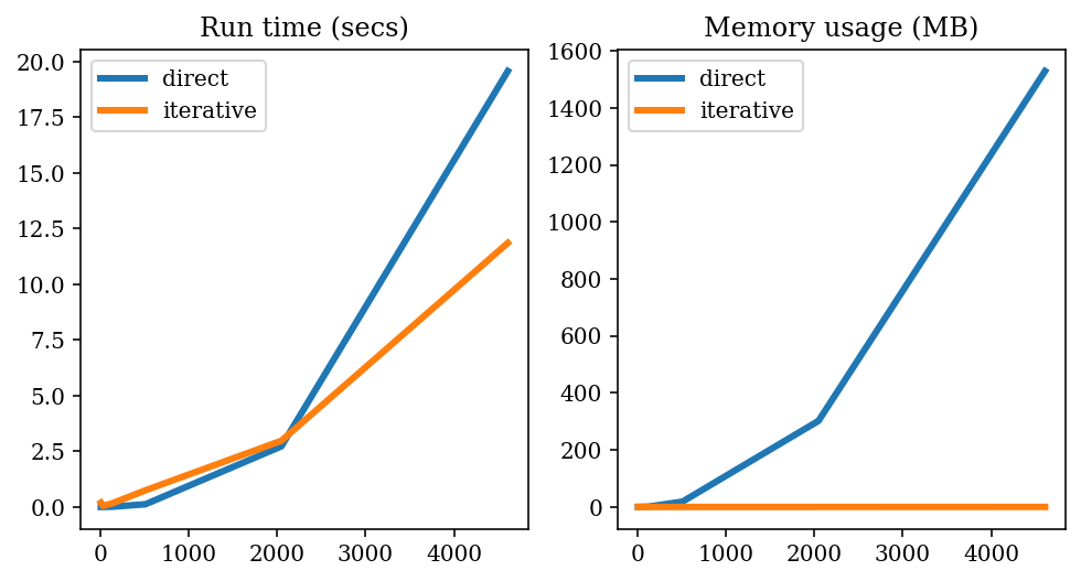
An important thing to note about the solution above is that only a few matrix-vector products are required to get to a high-level of accuracy. GMRES (and many other iterative linear and nonlinear optimization algorithms) converges at a rate proportional to the condition number of the matrix [Saad and Schultz, 1986]. So in order to productively use an iterative linear solver, we need to have a matrix with a small condition number. It turns out that these free surface self-interaction matrices have condition numbers that are very close to 1.0, meaning that all the eigenvalues are very similar in magnitude. As a result, a highly accurate solution with GMRES requires less than ten matrix-vector products even for very large matrices.
Because of this dependence on the condition number, in the worst case, iterative solvers are not faster than a direct solver. However, suppose that we need only 10 matrix-vector products. Then, the runtime is approximately \(10(2n^2)\) because each matrix-vector product requires \(2n^2\) operations (one multiplication and one addition per matrix entry). As a result, GMRES is solving the problem in \(O(n^2)\) instead of the \(O(n^3)\) asymptotic runtime of direct methods like LU decomposition. So, in addition to requiring less memory, the matrix free method here forced us into actually using a faster linear solver. Of course, LU decomposition comes out ahead again if we need to solve many linear systems with the same left hand side and different right hand sides. That is not the case here but would be relevant for many other problems (e.g. problems involving time stepping).
The mess of code below builds a few figures that demonstrate these points regarding performance and accuracy as a function of the number of elements.
import time

fault_L = 1000.0
fault_H = 1000.0
fault_D = 0.0
fault_pts = np.array(
    [
        [-fault_L, 0, -fault_D],
        [fault_L, 0, -fault_D],
        [fault_L, 0, -fault_D - fault_H],
        [-fault_L, 0, -fault_D - fault_H],
    ]
)
fault_tris = np.array([[0, 1, 2], [0, 2, 3]], dtype=np.int64)

results = []
for n_els_per_dim in [2, 4, 8, 16, 32, 48]:
    surf_L = 4000
    mesh_xs = np.linspace(-surf_L, surf_L, n_els_per_dim + 1)
    mesh_ys = np.linspace(-surf_L, surf_L, n_els_per_dim + 1)
    mesh_xg, mesh_yg = np.meshgrid(mesh_xs, mesh_ys)
    surf_pts = np.array([mesh_xg, mesh_yg, 0 * mesh_yg]).reshape((3, -1)).T.copy()
    surf_tris = []
    nx = ny = n_els_per_dim + 1
    idx = lambda i, j: i * ny + j
    for i in range(n_els_per_dim):
        for j in range(n_els_per_dim):
            x1, x2 = mesh_xs[i : i + 2]
            y1, y2 = mesh_ys[j : j + 2]
            surf_tris.append([idx(i, j), idx(i + 1, j), idx(i + 1, j + 1)])
            surf_tris.append([idx(i, j), idx(i + 1, j + 1), idx(i, j + 1)])
    surf_tris = np.array(surf_tris, dtype=np.int64)
    surf_tri_pts = surf_pts[surf_tris]
    surf_centroids = np.mean(surf_tri_pts, axis=1)

    fault_surf_mat = cutde.disp_matrix(surf_centroids, fault_pts[fault_tris], 0.25)
    rhs = np.sum(fault_surf_mat[:, :, :, 0], axis=2).flatten()

    start = time.time()
    eps_mats = []
    offsets = [0.002, 0.001]
    offset_centers = [
        np.mean(surf_tri_pts, axis=1) - off * np.array([0, 0, 1]) for off in offsets
    ]
    for i, off in enumerate(offsets):
        eps_mats.append(cutde.disp_matrix(offset_centers[i], surf_pts[surf_tris], 0.25))
    lhs = 2 * eps_mats[1] - eps_mats[0]
    lhs_reordered = np.empty_like(lhs)
    lhs_reordered[:, :, :, 0] = lhs[:, :, :, 1]
    lhs_reordered[:, :, :, 1] = lhs[:, :, :, 0]
    lhs_reordered[:, :, :, 2] = lhs[:, :, :, 2]
    lhs_reordered = lhs_reordered.reshape(
        (surf_tris.shape[0] * 3, surf_tris.shape[0] * 3)
    )
    lhs_reordered += np.eye(lhs_reordered.shape[0])
    direct_build_time = time.time() - start
    start = time.time()
    soln = np.linalg.solve(lhs_reordered, rhs).reshape((-1, 3))
    direct_solve_time = time.time() - start

    def matvec(x):
        extrapolation_mult = [-1, 2]
        slip = np.empty((surf_centroids.shape[0], 3))
        xrshp = x.reshape((-1, 3))
        slip[:, 0] = xrshp[:, 1]
        slip[:, 1] = xrshp[:, 0]
        slip[:, 2] = xrshp[:, 2]
        out = np.zeros_like(offset_centers[0])
        for i, off in enumerate(offsets):
            out += extrapolation_mult[i] * cutde.disp_free(
                offset_centers[i], surf_tri_pts, slip, 0.25
            )
        return out.flatten() + x

    n = surf_tris.shape[0] * 3

    def M(x):
        M.n_iter += 1
        return matvec(x)

    M.n_iter = 0
    lhs = spla.LinearOperator((n, n), M, dtype=rhs.dtype)
    start = time.time()
    soln_iter = spla.gmres(lhs, rhs, tol=1e-4)[0].reshape((-1, 3))
    iterative_runtime = time.time() - start

    l1_err = np.mean(np.abs((soln_iter - soln) / soln))
    results.append(
        dict(
            l1_err=l1_err,
            n_elements=surf_tris.shape[0],
            iterations=M.n_iter,
            direct_build_time=direct_build_time,
            direct_solve_time=direct_solve_time,
            iterative_runtime=iterative_runtime,
            direct_memory=rhs.nbytes + lhs_reordered.nbytes,
            iterative_memory=rhs.nbytes,
        )
    )
import pandas as pd

results_df = pd.DataFrame({k: [r[k] for r in results] for k in results[0].keys()})
results_df["direct_runtime"] = (
    results_df["direct_build_time"] + results_df["direct_solve_time"]
)
results_df
| l1_err | n_elements | iterations | direct_build_time | direct_solve_time | iterative_runtime | direct_memory | iterative_memory | direct_runtime | |
|---|---|---|---|---|---|---|---|---|---|
| 0 | 0.000390 | 8 | 6 | 0.001730 | 0.000297 | 0.196446 | 4800 | 192 | 0.002027 |
| 1 | 0.000052 | 32 | 7 | 0.001941 | 0.000353 | 0.045686 | 74496 | 768 | 0.002294 |
| 2 | 0.000371 | 128 | 7 | 0.007796 | 0.001663 | 0.152800 | 1182720 | 3072 | 0.009458 |
| 3 | 0.000520 | 512 | 7 | 0.085798 | 0.037337 | 0.748936 | 18886656 | 12288 | 0.123135 |
| 4 | 0.000599 | 2048 | 7 | 1.271554 | 1.452238 | 2.974715 | 302039040 | 49152 | 2.723793 |
| 5 | 0.000887 | 4608 | 7 | 6.120567 | 13.449475 | 11.854967 | 1528934400 | 110592 | 19.570042 |
plt.rcParams["text.usetex"] = False
plt.figure(figsize=(8, 4))
plt.subplot(1, 2, 1)
plt.plot(results_df["n_elements"], results_df["direct_runtime"], label="direct")
plt.plot(results_df["n_elements"], results_df["iterative_runtime"], label="iterative")
plt.legend()
plt.title("Run time (secs)")
plt.subplot(1, 2, 2)
plt.plot(results_df["n_elements"], results_df["direct_memory"] / 1e6, label="direct")
plt.plot(
    results_df["n_elements"], results_df["iterative_memory"] / 1e6, label="iterative"
)
plt.legend()
plt.title("Memory usage (MB)")
plt.show()